Population structure

Motivation

Phylogenetic clustering is one method to group individuals together. However, these methods often make strong assumptions, for example that individual genotypes are related by strictly bifurcating genealogical or phylogenetic processes. These assumptions are often violated, particularly in crop species with their complex phylogentic history. For this reason, different methods for the analysis of genetic similarity, relatedness and population structure are used.

Population genetics theory provides many models for investigating population structure and migration between populations. These models assume, however, that the population structure is known.

In the analysis of real populations, the exact population structure is usually unknown. A population structure can be defined in several ways:

• Geographic origin
• Phenotypic similarity
• Genetic similarity

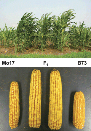
Frequently, geographic origin or phenotypic similarity may be used to make reasonable assumptions about population structure, but such assumptions can be misleading. High rates of migration or seed exchange may lead to a mixing of genetic variation within the distribution range of a species, and the geographic information may not indicate genetic similarity anymore. Phenotypic differences are frequently correlated with average genome-wide genetic distance. Phenotypically different individuals may have a high level of genetic similarity except in a few genes that are responsible for a few conspicuous traits. For example, more than 90% of the genetic variation in the human population is contained within populations, and only a relatively small proportion of genes such as those controlling skin color are highly differentiated between human populations. On the other hand, phenotypically similar individuals may be characterized by a high level of genetic diversity. A case in point are maize inbred lines, such as Mo17 and B37. Phenotypically, the look quite similar (Table 1 and Figure 1), but a F1 hybrid resulting from a cross of the two parents has larger trait values for many traits, which indicates heterosis that reflects genetic differences between the parents.

Table 1: Phenotypic differences between the two North American maize inbred lines Mo17 and B73. Source: Springer and Stupar (2007)

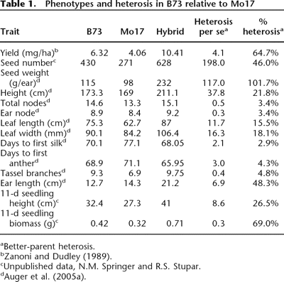
Since it is known that heterosis is correlated with the genetic distance between two individuals (Reif et al., 2003), it can be used to estimate genetic distance between individuals. The high genetic diversity between the two is confirmed by the sequencing of the bronze region, which is highly divergent between the two inbred lines.

Figure 1: Phenotypic differences between the two parental lines Mo17 and B73 and their hybrid offspring. Source: Springer and Stupar (2007)

To conclude, an estimation of genetic similarities is more correct than phenotypic or geographic estimates in the context of plant breeding. Several methods are available for inferring population structure. The most frequently used methods are phylogenetic analysis, principle components analysis and model-based inference.

Phylogenetic analysis

The basics of phylogenetic analysis were described before, and shown to be a powerful method for identifying individuals that are closely related and to identify groups of individuals. One disadvantage is, however, that frequently it is difficult to identify the exact number of distinct groups in a sample. An example is shown in a study of maize domestication.

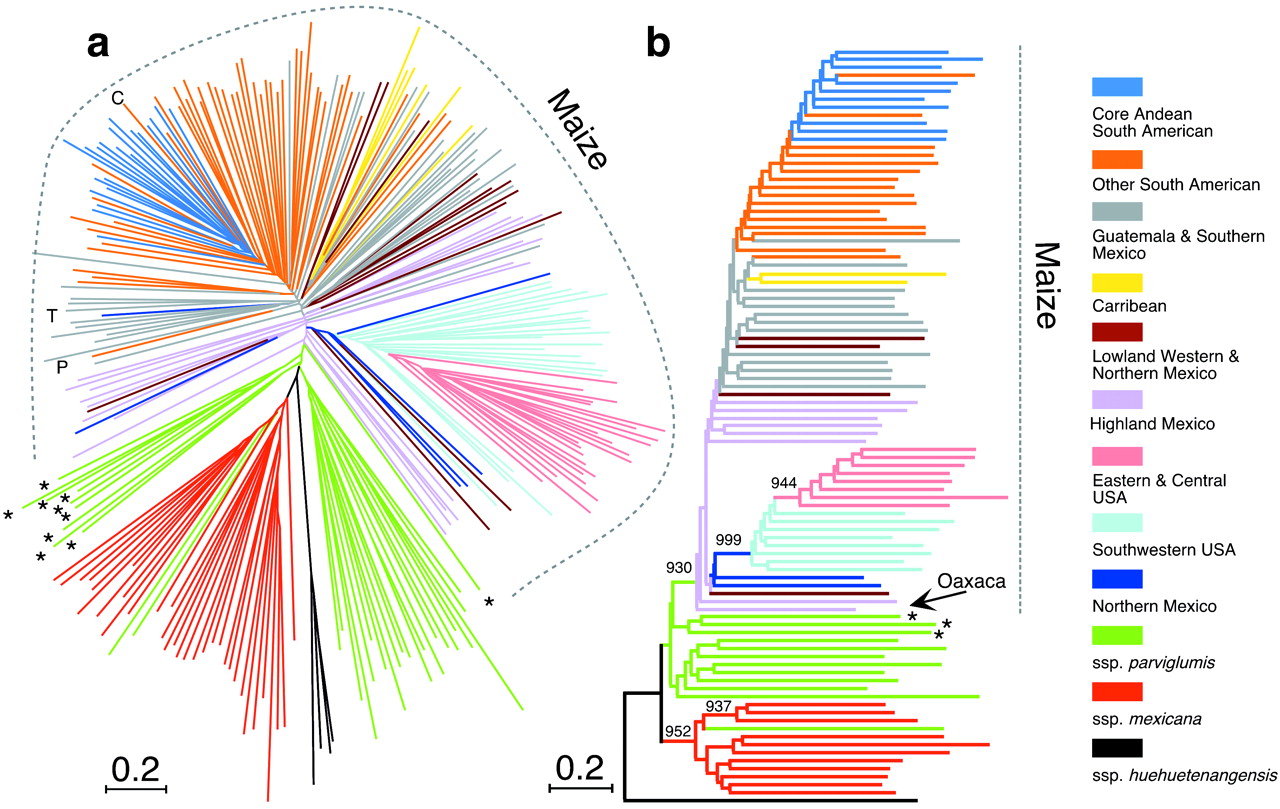
A set of 264 plants were genotyped with 99 simple sequence repeats (SSR) as genetic markers (Matsuoka et al., 2002) and analyzed with phylogenetic methods. The tree is characterized by large terminal branches, and only few internal branches with significant bootstrap support (Figure 2). In summary, the tree supports the grouping of North American groups, but the clustering of the accessions from Mexico and the rest of Latin America is not supported statistically. It is therefore difficult to identify accessions that are representative for particular subpopulations based on the microsatellite markers.

Figure 2: Phylogenetic analysis of American maize germ plasm using SSR markers. (A) Unrooted tree. (B) Rooted tree. Source: Matsuoka et al. (2002)

Principal components analysis (PCA)

Principle component analysis, or PCA has been used for a long time in population genetics to cluster related groups of individuals. PCA is a method to reduce the dimensions of complex multivariate data to identify key components of the structure within the data in a model-free manner. Its key feature is to project samples onto a series of orthogonal axes, each of which is made up of a linear combination of allelic or genotypic values across markers. The goal of a PCA analysis is to project the data on a first axis that contains the highest proportion of variation in the data. Then it moves to the second axis to maximize the variance for all possible axes perpendicular to the first axis, and so on. Usually, only the first two or three axis are presented, but a PCA analysis can comprise more axes.

To summarize, PCA

• is a model-free and a parameter-free approach
• finds different combinations of markers such that these combinations are uncorrelated. These combinations are called principal components.
• explains the total variation in the data as the sum of all principal components
• is computationally fast
• is able to identify structures in the sample caused by a diversity of evolutionary processes

To reduce complexity among principal components, only a small number of components that explain the highest proportion of total variation is retained because they usually can be used to investigate the most important patterns in the data.

A brief description of PCA

PCA was described by Karl Pearson in 1901 and it was first used in population genetics by Menozzi et al. (1978). The goal of PCA is to take \(n\) variables \(X_1,X_2,X_3,\ldots,X_n\) and to find combinations of these variables that produce indices \(Z_1,Z_2,\ldots,Z_n\) that are uncorrelated. In our case, \(X_i\) is marker \(i\). Since the indices \(Z\) are uncorrelated, they measure different ‘dimensions’ in the data (i.e., they are orthogonal to each other).

The indices can be ordered, so that \(Z_1\) explains the largest amount of variation in the data, \(Z_2\) the second largest, and so on.

The \(Z_i\) indices are called principal components. One goal of PCA is to identify those principal components, which explain a large proportion (i.e., 90%) of the variation in the data. If the \(n\) original \(X\) variables can be reduced to a smaller number of variables, then confounding factors between data can be excluded, such as a correlation of allele frequencies at different markers that may be caused by the presence of population structure.

The steps in PCA are as follows:

1. Code variables \(X_1,X_2,\ldots,X_n\) such that they have mean zero and variance 1.
2. Calculate the covariance matrix between all pairwise combinations of variables. If the variables are normalized (as in step 1), the matrix is a correlation matrix.
3. Calculate the eigenvalues, \(\lambda_1,\lambda_2,\ldots,\lambda_n\) of each variable, and the corresponding eigenvectors \(\mathbf{a_1, a_2, \ldots, a_n}\).¹
4. The coefficient of the \(i\)-th principal component are then given by \(\mathbf{a_1}\), and \(\lambda_i\) gives its variance. Principal components can be ordered by their variance.

¹ Eigenvalues and eigenfactors are fairly complex theorems of matrix algebra, which we do not discuss further here.

More detailed technical descriptions of principal components analysis can be found in many sources such as in Manly (2005), and there are computer programs available to conduct PCA (or related multivariate statistics) on genetic or phenotypic data.

Applications of PCA in the context of plant genetic resources

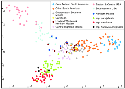
The same data as in Figure 2 are shown in Figure 3. Several aspects become obvious:

1. Accessions from geographically close regions cluster together, but we do not have a measure of statistical significance of the association.
2. The two axes of the plot are dimensionless; only the proximity in the two dimensions indicates similarity.
3. Maize accessions (as opposed to the close relatives) are spread mainly over the first principal component (\(x\) axis) indicating that most of the variation covered by the first axis is almost entirely due to variation in cultivated maize.
4. The second principal component (y-axis) separates the wild ancestors from cultivated maize.
5. The total amount of variation present in the first two principal components is only 3.5 \(+\) 2.6 \(=\) 6.1% of the variation. Hence, the overall extent of geographic structure is low and most alleles can be found throughout the distribution range ²
6. The wild relatives are located close to the Mexican landraces which supports the hypothesis that domestication occurred in Mexico. North and South American landraces appear to have experienced largely independent evolutionary trajectories as they are roughly ordered according to the geographic latitude from North to South along the \(x\) axis.

² A lack of a strong geographic structure also causes the short internal branch lengths of the phylogeny in Figure 2

Figure 3: Graph of the first two axes from a principal component analysis of 193 maize and 71 teosinte individual plants. The first component explains 3.5% and the second 2.6% of the total variation. Source: Matsuoka et al. (2002)

In recent years, simulation studies and theoretical analyses showed that despite its age, PCA is still a useful technique:

1. It is possible to interprete principal components in terms of gene genealogies as formulated by coalescence theory and to identify different evolutionary processes that influenced genetic variation (McVean, 2009).
2. It provides information about the effects of uneven sampling of individuals on patterns of genetic variation in the sample (McVean, 2009).
3. It can be interpreted in a geographic context to identify the role of demographic processes like bottlenecks, migration and range expansion (Novembre and Stephens, 2008).
4. The number of relevant principal components can be evaluated statistically to identify the number of distinct genetic clusters in the data (Patterson et al., 2006).

Because of these characteristics, PCA will continue to play an important role in future analyses of genetic variation.

Model-based inference

The STRUCTURE approach

An third approach to analysing population structure is based on an explicit model of a population structure and evolution. The most frequently used implementation of such a model is the STRUCTURE program (Pritchard et al., 2000) and variants of this program that differ in their implementation and model assumptions. The basic model of STRUCTURE assumes that alleles within a population are in Hardy-Weinberg equilibrium and that all markers are in complete linkage equilibrium within populations. It is assumed that any deviation from HWE and a presence of linkage disequilibrium results from population structure. The program tries to find population groupings of individuals that minimize the level of disequilibrium within populations and maximizes the fit to the expected HWE given the allele frequencies of markers used.

The STRUCTURE algorithm uses a probabilistic approach to infer the population structure that is most consistent with the data. Two modifications of the model are possible. In a model without admixture, each individual is assigned to a single population, and in a model with admixture, individuals are allowed belong to different populations (i.e., 50% to population 1 and 50% to population 2). To infer the number of populations, the population is run with different values of \(K\), which corresponds to the number of populations in the model. Then, for each \(K\), the likelihood of the data given a value of \(K\), \(P(X|K)\) is calculated. Inferring the number of clusters \(K\) that explains the data best is difficult, but several good algorithms are available and should be used (just choosing the \(K\) with the highest likelihood is not optimal).³ The program then assigns each individual to a population. If the model with admixture is chosen, an output matrix, \(Q\) is produced that assigns each individual proportionally to each of the \(K\) populations. The assignment can be visualized graphically.

³ See the tutorial of Lawson et al. (2018) for details

Each individual in the sample corresponds to a vertical line, and the proportional population assignment is expressed by different colors. Admixed individuals are recognizable if they show more than one color. As an example, the STRUCTURE analysis of cultivated barley that were genotyped with \(16\) SSR markers (Figure 4) (Stracke et al., 2007).

Figure 4: Example of a STRUCTURE analysis in barley genetic resources. The population structure is based on the analysis of 16 SSR markers. Source: stracke_effects_2007

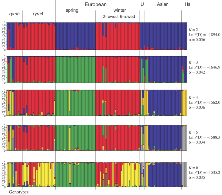
The figure shows that with different values of \(K\) the subpoplations present in the material can be differrentiated. Vor example with \(K=2\) the European winter and spring barley types can be differentiated. The analysis also reveals that all genotypes that contain the rym4 gene against Barley Yellow Mosaic Virus are genetically very similar to the winter type. The analysis with \(K=6\) indicates separate clusters for the 2-rowed and 6-rowed winter barley types.

In summary, STRUCTURE has several noteworthy aspects:

• Due to the algorithm for evaluating the different groups of individuals, STRUCTURE may have long running times, especially with large datasets.
• Several alternative implementations of STRUCTURE are available. We recommend using ADMIXTURE (Alexander et al., 2009), which is availabe here http://software.genetics.ucla.edu/admixture/index.html
• Like PCA, STRUCTURE is strongly influenced by unequal sampling. Missing populations (‘Ghost populations’) may lead to wrong inference (Beerli, 2004).
• Simulation studies showed that STRUCTURE tends to produce the highest level ordering of populations. Subpopulations within larger populations need to be identified by re-running STRUCTURE with only the individuals of a given population (Evanno et al., 2005).

The ADMIXTURE approach

Since ADMIXTURE has some favorable properties, it will be briefly explained in the following:

Like STRUCTURE it assumes that each subpopulation is in Hardy-Weinberg equilibrium (HWE) and all markers are in complete linkage equilibrium within populations. It uses, however, a Maximum likelihood approach to infer population structure.

First, individuals are rearranged to maximize fit to HWE. This step is done for different numbers of populations, \(K\). Then, likelihood of data for each \(K\) are calculated and \(K\) with the highest likelihood is selected.

In the next step, each individual is proportionally assigned to each population using the following algorithm. Assume that the sample contains genetic material inherited from \(K\) ancestral populations, which had allele frequencies \(A=(A_{i,1}\ldots,A_{i,K})\) at the observed loci \(i\). Then, for each individual assume that a fraction of \(q_j\) its DNA can be traced back to the $j$th (ancestral) populations. Calculate likelihood of the genetic data of each individual being produced from \(K\) subpopulations with the assumed \(q\) and \(A\) for every possible choice of \(q\) and \(A\). Take the ancestry fractions \(q\) that produce the highest likelihood.

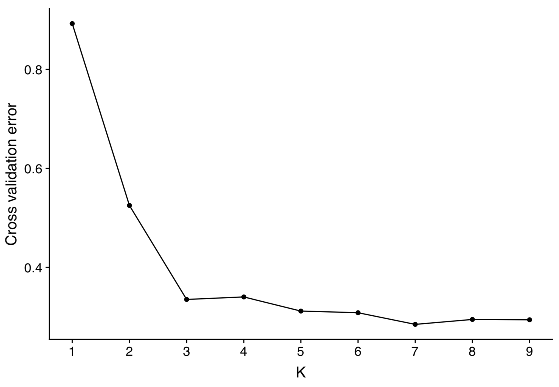
To choose the best-fitting \(K\) value, cross-validation is frequently used. Cross-validation is a widely used method to infer the robustness of model selection and parameter estimation obtained from a data set. First, mask a proportion of the SNP matrix (e.g. SNP position 5 in individual 3,…) at random. Estimate ancestries and ancestral allele frequencies without the masked information. Then, predict the masked entries and record the error. After repeating these steps multiple times, select the \(K\) value with the smallest error averaged over multiple cross-validations.

An example of this procedure is shown in Figure 5 from a study of population structure in amaranths (Stetter et al., 2020). It shows a substantial reduction of the cross-validation error until \(K=3\), and with higher \(K\) values, it remains essentially constant, although one may select \(K=7\) as the best value. The decision on which \(K\) value to choose frequently is not only guided by statistical arguments, but also involves biological knowledge. In this particular case, for example \(K=7\) is highly plausible because it includes three strongly differentiated subpopulations of the wild ancestor species, another very closely related wild ancestor species and the three distinct grain amaranth species.

Figure 5: Cross-validation plot resulting from an ADMIXTURE analysis. Usually the \(K\) value with the smallest absolute value is chosen as best-fitting model. Source: (Stetter et al., 2020).

Synopsis population structure inference

There are many more methods for population structure available then the ones presented, although frequently they are modifications of phylogenetic, PCA or model-based approaches. If the data are robust and sufficient in terms of marker numbers and sample size, the three methods converge towards the same results, although each method allows to investigate additional aspects of the data such as admixture or gene flow.

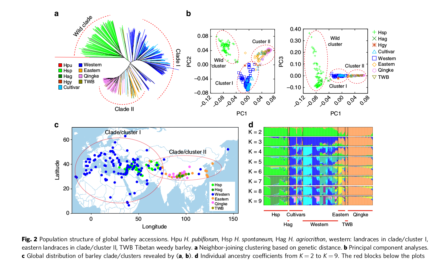
Figure 6 shows a comparison of the three methods, which confirms the notion that major patterns in the data are usually found by different methods. In this particular case, it is the strong genetic differentiation between wild and domesticated, and between barley landraces from the western distribution range (Near East, Europe, North Africa) and the Eastern distribution range (Tibet).

Figure 6: Population structure of global barley accessions. Source: Zeng et al. (2018)

Key concepts

\(\square\) Population structure inference

\(\square\) Principal components analysis (PCA)

\(\square\) Model-based inference

Summary

• The analysis of population structure is an important aspect of the study of genetic resources.
• Several methods for population structure analysis exist that include phylogenetic analysis, principal components analysis and model-based inference such as the STRUCTURE method.
• A phylogenetic approach is usually fast and robust, however it does not provide well defined criteria for population subdivision and the assignment of individuals to populations.
• Principle component analysis is a fast and reliable method. It is not based on a model of evolution, but recent improvements facilitate statistical analysis and an interpretation of results in the context of evolutionary processes.
• Model-based approaches such as the STRUCTURE program allow to estimate the number of populations and to assign individuals to different populations. Unfortunately, this method can be slow, which is problematic for large data sets. More recent implementations have greatly accelerated model-based structure analysis.

Further reading

• Lawson et al. (2018) - This is a good introduction into interpreting STRUCTURE-type plots of population structure analyses.
• Novembre and Peter (2016) - Short review on the analysis of fine-scaled population structure (in humans)

Review and thinking questions

1. Which type of information can be used to group plant genetic resources? What is the advantage and disadvantage of each type of information?
2. What are he major methods for population inference, and what are there characteristics?
3. Why is it often necessary to infer the population genetic structure of genetic resources?
4. Do self-fertilizing crops such as wheat meet the requirements of a STRUCTURE analysis? (Hint: think about HWE).

Problems

1. Both (Matsuoka et al., 2002) and Heerwaarden et al. (2011) analysed a large panel of American maize landraces with PCA. However, the two studies used different markers (SSRs versus SNPs). A key difference between SSRs is that each marker tends to have multiple alleles, whereas SNPs usually have 2 markers. Compare the PCA plots in both studies: What do they have in commom with respect to the population structure of American maize genetic diversity, and where do they differ?
2. Stetter et al. (2020) investigated the genetic relationship of wild amaranths and three species of domesticated grain amaranths from South and Central America using phylogenetic trees, PCA and Structure analyses. Download the publication and the supplementary material and compare the tree (Supplement: S3), the PCA (Paper: Fig 1) and the ADMIXTURE (=STRUCTURE) analysis (Supplement: Fig S1). Do the three methods provide similar results with respect to the relationship of wild and domesticated amaranths? Open Supplementary file Sfig1.html in a browser and analyse the three-dimensional PCA plot. nWhich advantage do you see by having a 3D instead of a 2D plot?

In class exercises

Discussion questions

1. Which type of information can be used to group plant genetic resources? What is the advantage and disadvantage of each type of information?
2. Why is it often necessary to infer the population genetic structure of genetic resources?
3. Assume you use two different methods to analyse the population structure in your data set and the results disagree. What could be the reason? How can you decide which method to “trust” or what can you do?

Brasscia rapa domestication

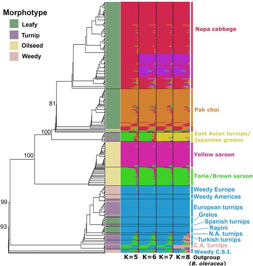
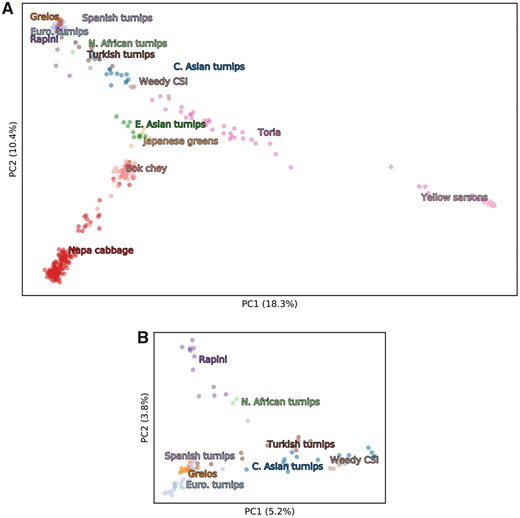
McAlvay et al. (2021) investigated the domestication history of Brassica rapa by analysing a diversity panel of 416 domesticated and weedy samples. They used different methods to investigate the population structure in their data set. Figures 1 and 2 show the results of their phylogenetic and model-based inference and of the PCA.

1. Look only at the phylogenetic tree in Figure 1. How many clusters can you identify? How well are the clusters or nodes supported?
2. Figure 1 also shows the results of a fastSTRUCTURE analysis (similar to STRUCTURE) from \(K=5\) to \(K=8\). Briefly describe how the pattern changes from \(K=5\) to \(K=8\). Can you identify any admixed samples and how are they admixed?
3. Compare the phylogenetic tree and the fastSTRUCTURE result in Figure 1. Do they agree or disagree?
4. Figure 2 shows the result of the PCA. Can you identify clusters? If yes, how many?
5. Compare the PCA to the results of the phylogenetic and model-based inference in Figure 1. Does the PCA agree or disagree with the phylogenetic and model-based inference? Assuming that the PCA does not agree: What could be a possible reason?

Figure 7: RAxML tree and fastSTRUCTURE plot indicating population structure of Brassica rapa crops and weeds at four different values of \(K\).

Figure 8: PCA displaying PCs 1 and 2 of Brassica rapa samples.

References

Alexander DH, Novembre J, Lange K. 2009. Fast model-based estimation of ancestry in unrelated individuals. Genome Research 19:1655–1664. doi:10.1101/gr.094052.109

Beerli P. 2004. Effect of unsampled populations on the estimation of population sizes and migration rates between sampled populations. Molecular Ecology 13:827–836. doi:10.1111/j.1365-294X.2004.02101.x

Evanno G, Regnaut S, Goudet J. 2005. Detecting the number of clusters of individuals using the software structure: A simulation study. Molecular Ecology 14:2611–2620. doi:10.1111/j.1365-294X.2005.02553.x

Heerwaarden J van, Doebley J, Briggs WH, Glaubitz JC, Goodman MM, Gonzalez J de JS, Ross-Ibarra J. 2011. Genetic signals of origin, spread, and introgression in a large sample of maize landraces. Proceedings of the National Academy of Sciences 108:1088–1092. doi:10.1073/pnas.1013011108

Lawson DJ, Dorp L van, Falush D. 2018. A tutorial on how not to over-interpret STRUCTURE and ADMIXTURE bar plots. Nature Communications 9:3258. doi:10.1038/s41467-018-05257-7

Manly B. 2005. Multivariate statistical methods, 3rd ed. Chapman & Hall/CRC.

Matsuoka Y, Vigouroux Y, Goodman M, Sanchez G, Buckler E, Doebley J. 2002. A single domestication for maize shown by multilocus microsatellite genotyping. Proc Natl Acad Sci USA 99:6080–6084. doi:10.1073/pnas.052125199

McAlvay AC, Ragsdale AP, Mabry ME, Qi X, Bird KA, Velasco P, An H, Pires JC, Emshwiller E. 2021. Brassica rapa Domestication: Untangling Wild and Feral Forms and Convergence of Crop Morphotypes. Molecular Biology and Evolution 38:3358–3372. doi:10.1093/molbev/msab108

McVean G. 2009. A Genealogical Interpretation of Principal Components Analysis. PLoS Genet 5:e1000686. doi:10.1371/journal.pgen.1000686

Menozzi P, Piazza A, Cavalli-Sforza L. 1978. Synthetic maps of human gene frequencies in Europeans. Science 201:786–792. doi:10.1126/science.356262

Novembre J, Peter BM. 2016. Recent advances in the study of fine-scale population structure in humans. Current Opinion in Genetics & Development, Genetics of human origin 41:98–105. doi:10.1016/j.gde.2016.08.007

Novembre J, Stephens M. 2008. Interpreting principal component analyses of spatial population genetic variation. Nature Genetics 40:646–649. doi:10.1038/ng.139

Patterson N, Price AL, Reich D. 2006. Population Structure and Eigenanalysis. PLOS Genetics 2:e190. doi:10.1371/journal.pgen.0020190

Pritchard JK, Stephens M, Donnelly P. 2000. Inference of Population Structure Using Multilocus Genotype Data. Genetics 155:945–959.

Reif J, Melchinger A, Xia X, Warburton M, Hoisington D, Vasal S, Srinivasan G, Bohn M, Frisch M. 2003. Genetic distance based on simple sequence repeats and heterosis in tropical maize populations. Crop Sci 43:1275–1282.

Springer NM, Stupar RM. 2007. Allelic variation and heterosis in maize: How do two halves make more than a whole? Genome Research 17:264–275. doi:10.1101/gr.5347007

Stetter MG, Vidal-Villarejo M, Schmid KJ. 2020. Parallel Seed Color Adaptation during Multiple Domestication Attempts of an Ancient New World Grain. Molecular Biology and Evolution 37:1407–1419. doi:10.1093/molbev/msz304

Stracke S, Presterl T, Stein N, Perovic D, Ordon F, Graner A. 2007. Effects of Introgression and Recombination on Haplotype Structure and Linkage Disequilibrium Surrounding a Locus Encoding bymovirus Resistance in Barley. Genetics 175:805–817. doi:10.1534/genetics.106.063800

Zeng X, Guo Y, Xu Q, Mascher M, Guo G, Li S, Mao L, Liu Q, Xia Z, Zhou J, Yuan H, Tai S, Wang Y, Wei Z, Song L, Zha S, Li S, Tang Y, Bai L, Zhuang Z, He W, Zhao S, Fang X, Gao Q, Yin Y, Wang J, Yang H, Zhang J, Henry RJ, Stein N, Tashi N. 2018. Origin and evolution of qingke barley in Tibet. Nature Communications 9:1–11. doi:10.1038/s41467-018-07920-5