Genetic mapping
Note: These notes need to be revised and made more concise.
Motivation
The phenotypic characterisation of PGR in field trials opens the possibility to identify genes, which influence interesting traits. Several types of methods are available for identifying underlying genes. They include linkage or QTL mapping based on crosses of few or multiple parents, or genome-wide association studies. Genome-wide association studies are a frequently used approach in genetic mapping because they use information of large numbers of accessions characterized in projects and are greatly facilitated by the sequencing or large-scale genotyping of genebank accessions.
In the following, genome-wide association studies are introduced as one approach for the characterization of plant genetic resources.
Identifiying large amount of associations problem that arises frequently in modern genomics data. The goal of genome-wide association studies (GWAS) is to unterstand the genetic of quantitative traits. In the following, we assume you have a basic understanding of the nature and characteristics of quantitative traits.
Studying the genetics of natural variation involves:
- Understanding the genetic architecture of traits of ecological and agricultural importance
- Identifying the genomic regions that control genetic variation
As genomics datasets become more common and sample sizes grow, the need for efficient statistical tests increases. GWAS tests for associations at many variants instead of some candidate genes and therefore hypothesis-free instead of hypothesis-driven with respect to the number and types of genes controlling phenotypic variation.
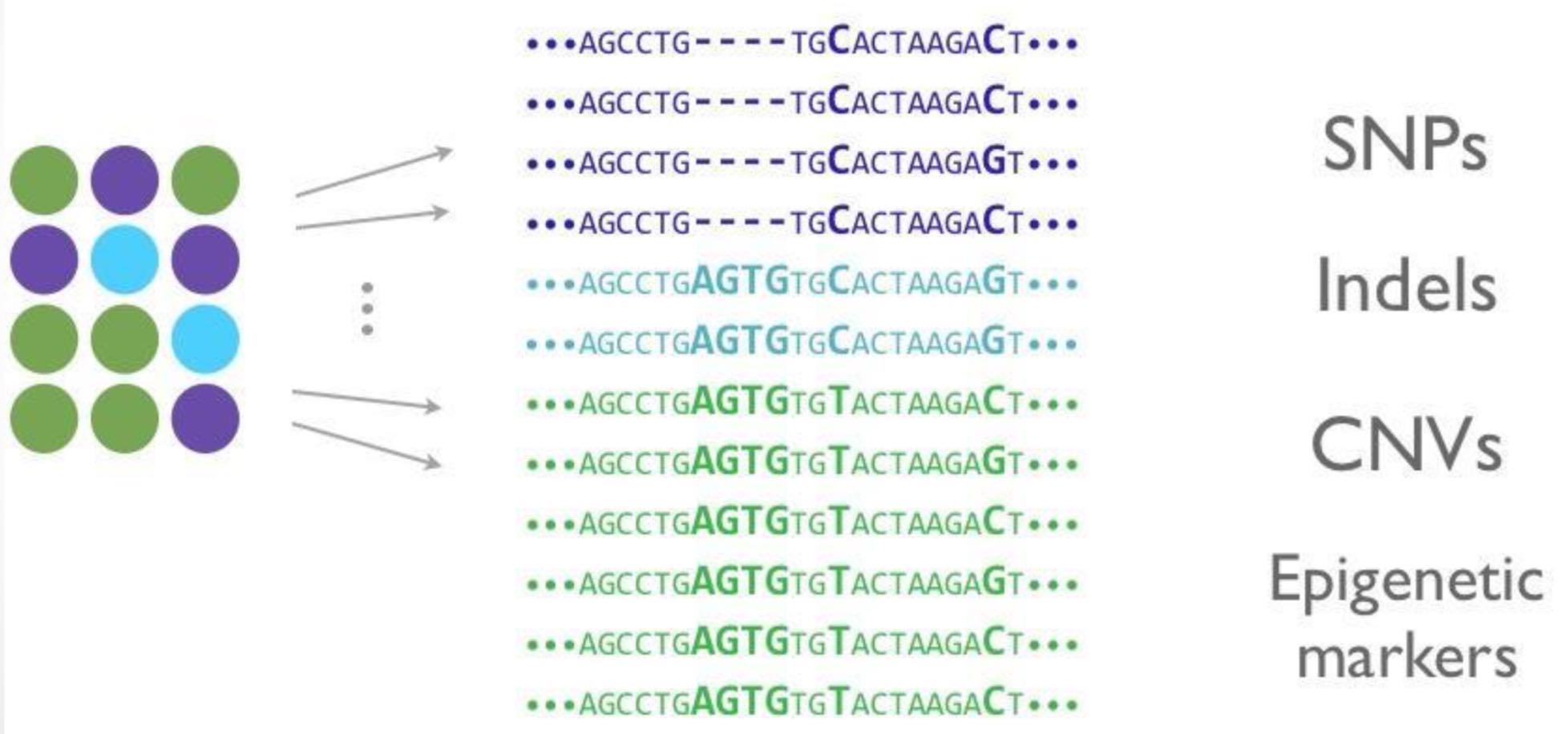
Figure 1 shows the key principle of GWAS: A set of plants (i.e., genebank accessions) are phenotyped. Phenotypic variation is indicated as the different colors. The same material is genotyped and the indivduals are ordered by their phenotypes. Associations between phenotypes and genotypic variation are identified using a statistical test.
In quantitative traits, both genes and the environment determine the phenotype. For this reason, a good experimental design needs to be employed to be able to differentiate between the two factors, and to allow the identification of the genotype on the phenotypic vcariation.
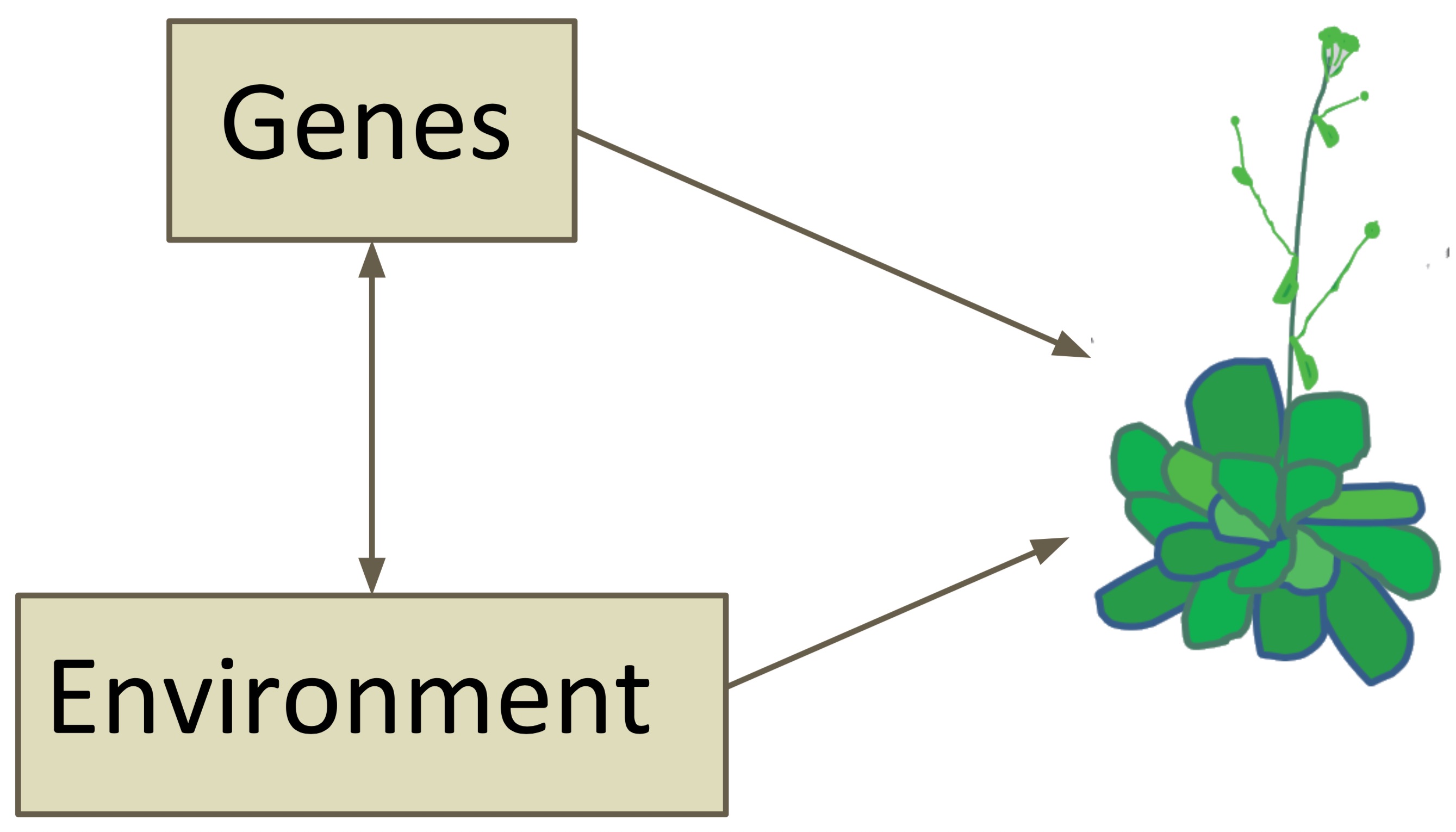
In particular, Genotype by Environment (GxE) provide a challenge because different traits are influenced by different degrees by the environment or by the genes.
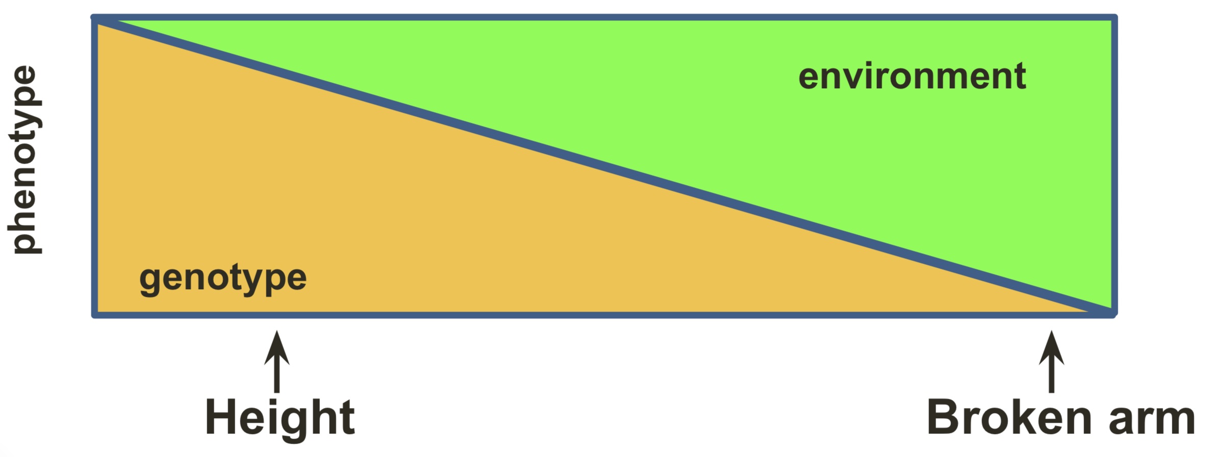
Figure 3 shows an example of a GWAS from the model plant Arabidopsis thaliana which allows to identify a genomic region that contains genetic variation for a trait in leaves.

Multiple testing problem
In GWAS a large number of marker tests are conducted, which leads to a multiple testing problem. Using a 5% significance threshold, we would expect 5% of the markers that have true marker effects of 0 to be significant in a statistical test of a null hypothesis. Bonferroni correction is a method for reducing the proportion of false positive. By assuming markers are independent we can obtain a conservative bound on the probability of rejecting the null hypothesis for one or more markers. \[\begin{equation} \label{bonferroni} 1-P(T_{1}\leq t, \ldots, T_{m} \leq t|H_{0}) \leq \alpha \end{equation}\] for a given significance threshold \(\alpha\). It should be noted, however, that the Bonferroni correction is overly conservative for a large number of tests and therefore leads to a high proportion of false negatives.
Other common methods include adjusted Bonferroni correction depending on rank, and permutations. However because of the statistical problems with the Bonferroni correction, other statistical approaches such as the use of the false discovery rate (FDR) have been proposed.
GWAS in plants
GWAS are important in plant research. In contrast to GWAS in humans, which are often highly critized, GWAS in plants have the advantage that appropriate experimental design reduces the environmental variance and the error. In addition, GWAS can be easily complemented by linkage mapping that is based on the analysis of crosses and their offspring.
A disadvantage of GWAS studies in plants is that they are often based on small sample sizes. Therefore the power to identify and estimate the effect of variants with small effect is difficult. For example the classical study by Atwell et al. (2010) was based on 107 individuals only.
Meanwhile, for model plants like A. thaliana and model crops like rice or maize, numerous resources are available that allow to download and (re-)analyse data using GWAS.
Linkage disequilibrium
Neighboring markers will tend to be inherited together, causing linkage disequilibrium (LD) between the two markers (Figure 4).
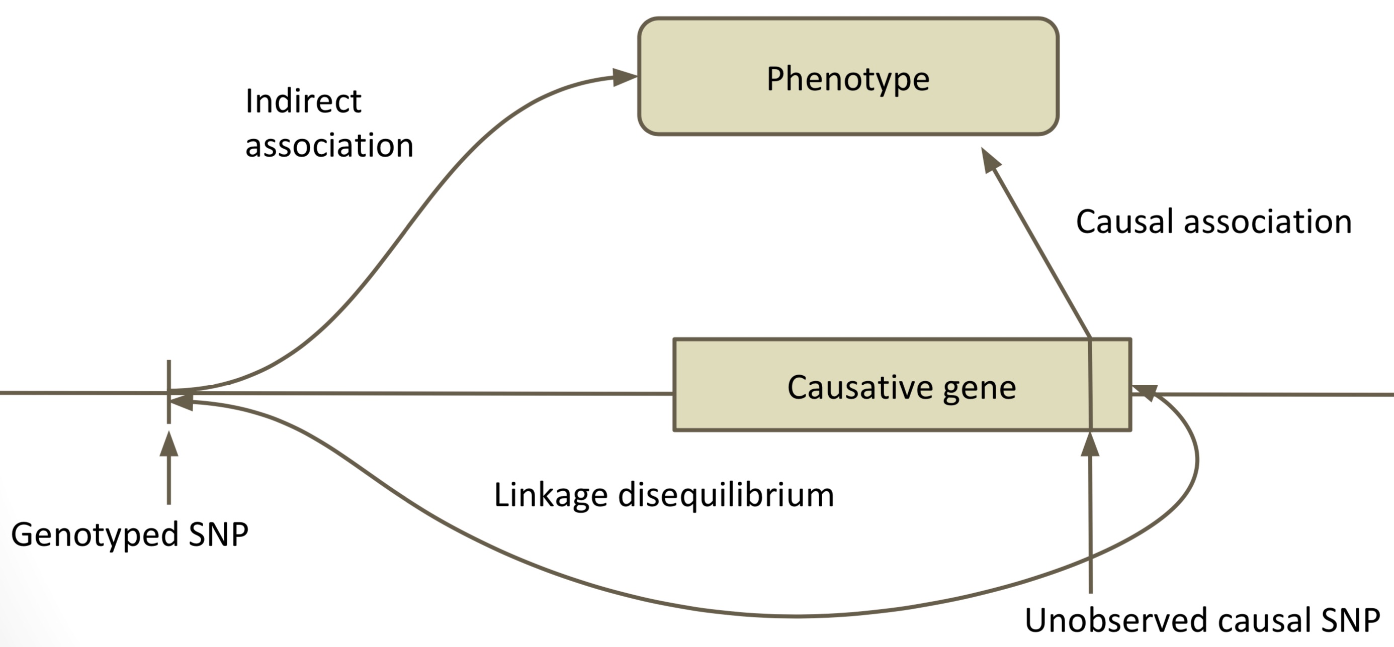
Since LD causes correlations between markers, in a given population we expect a lot of redundancy in the genotypes. LD is voth and advantage and disadvantage at the same time GWAS. The advantage is that linked markers are sufficient to identify an association with a QTL, on the other hand it makes is difficult to identify the causal variant if too many markers in the vicinity are linked to the causal variant.
Because of LD there is an important relationship between marker numbers and sample size to consider because both determine the resolution of GWAS. This relationship is strongly influenced by the genome-wide level of LD.
Population structure
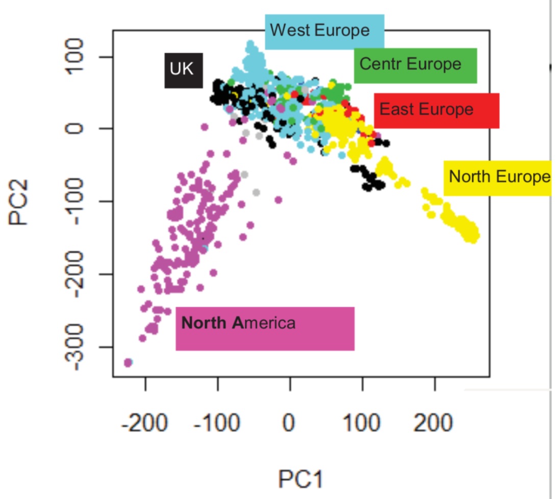
In natural populations, individuals tend to cluster in sub-populations according to their geographic origin. Methods for the inference of population structure like principal components analysis (PCA) (Figure 5) allow to identify subpopulations.
Confounding due to population structure may arise if it correlates with the trait in question (Figure 6)
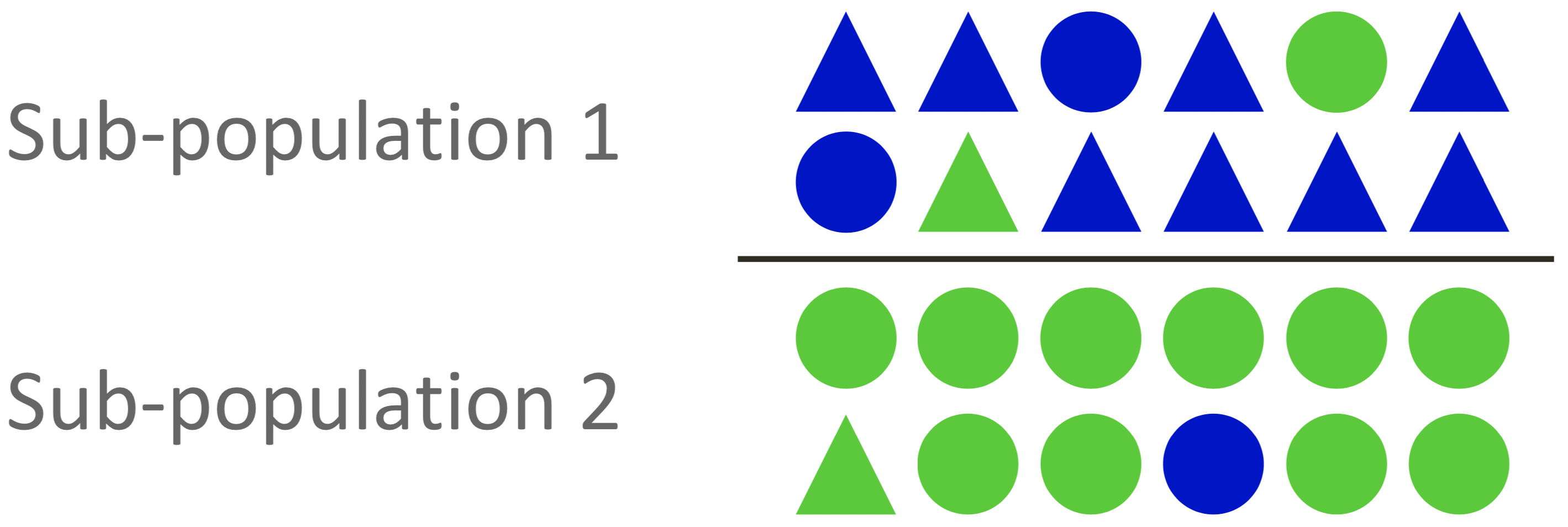
Any variant which is fixed for different alleles in each sub- population will show an association.
- Humans
- Genetic marker for skin color may also be associated with malaria resistance because the trait is correlated with population structure.
- Arabidopsis thaliana
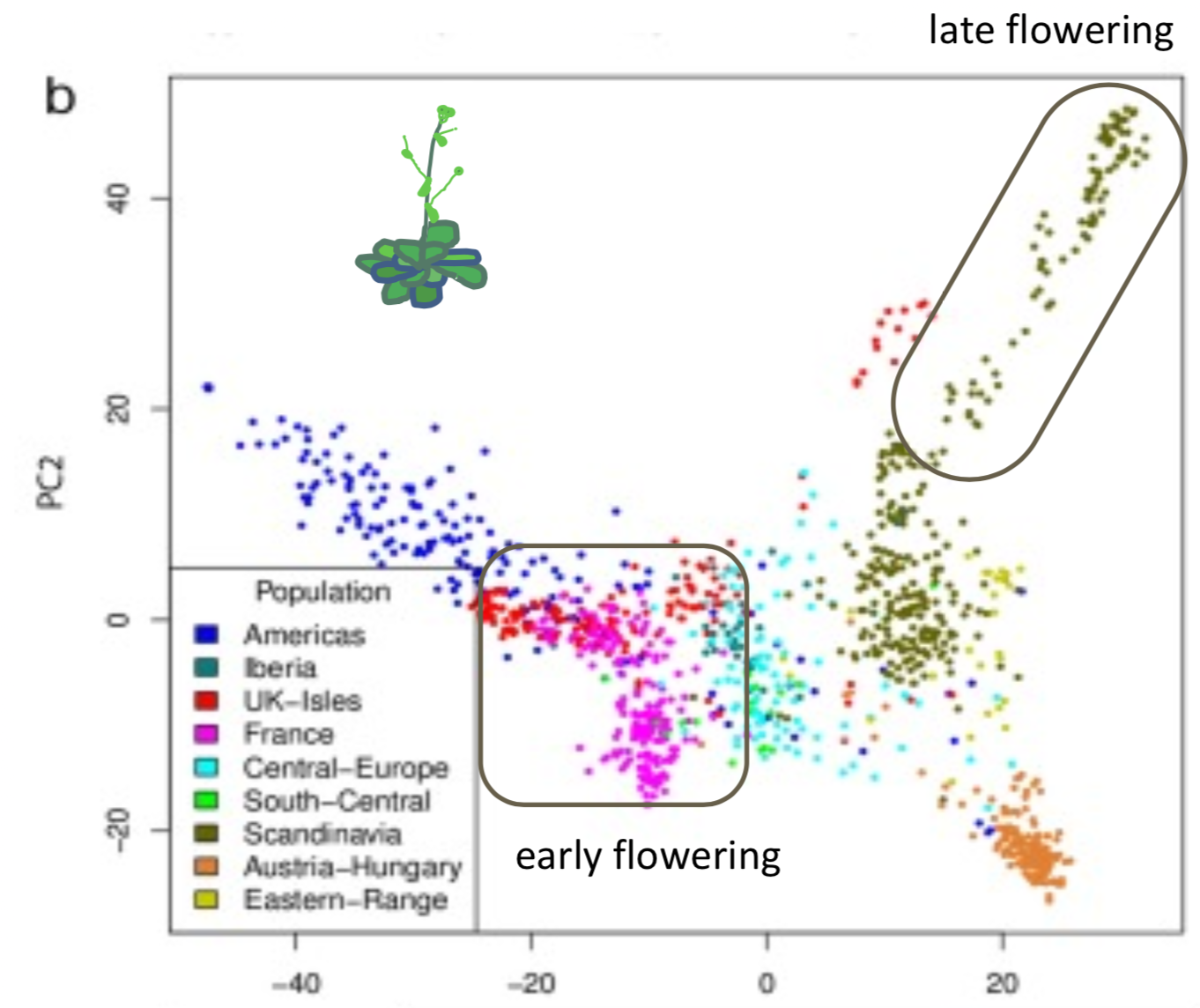
- Flowering time is correlated with latitude (Figure 7).
Disease resistance is not correlated with latitude.
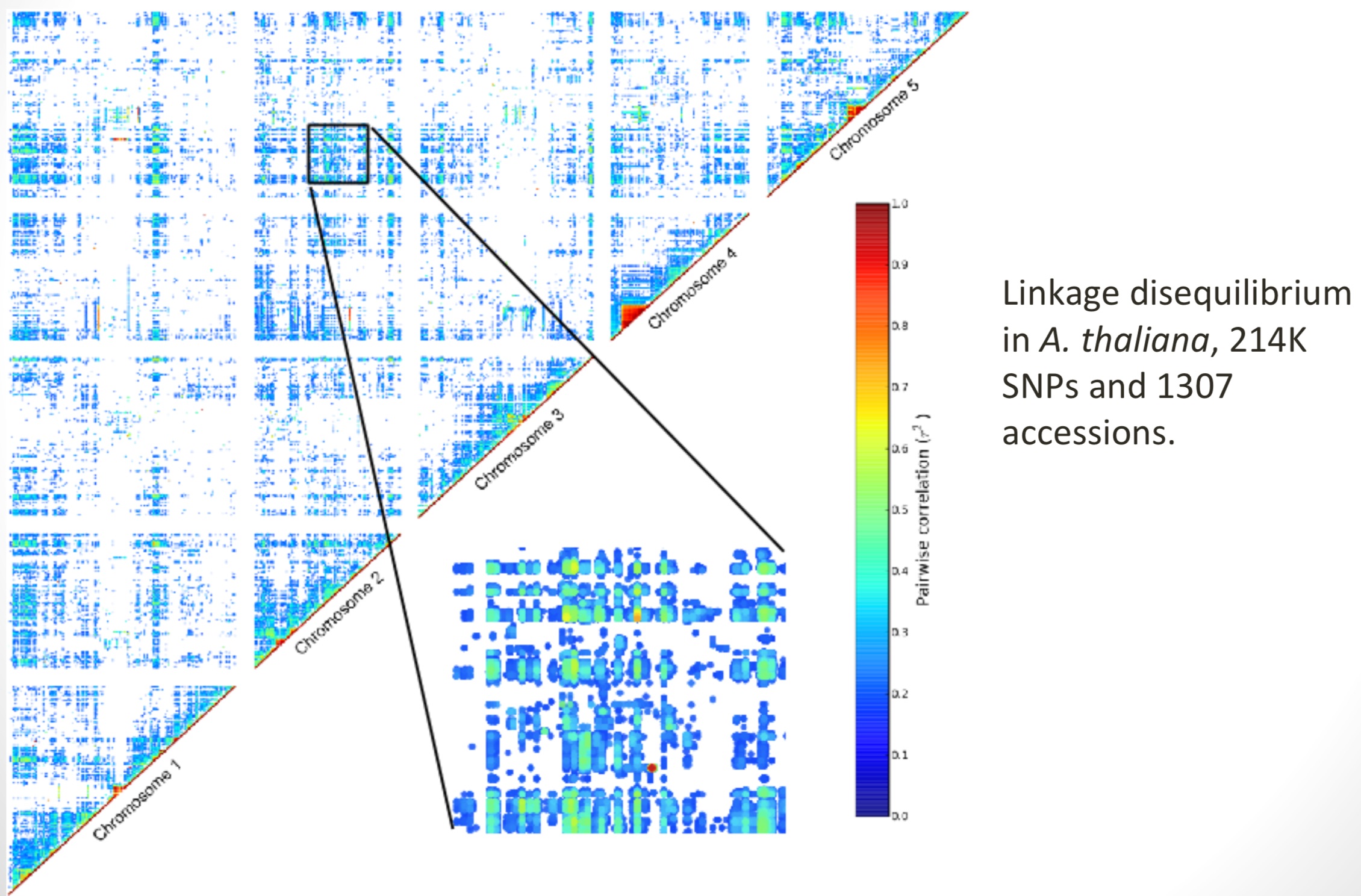
Population structure is reflected in long-range LD: A strong population structure in a sample also leads to long-range LD in the sample (Figure 8).
Implications for association studies:
- Test statistics is inflated
- High false positive rate
For this reason GWAS studies require a control to reduce the confounding of marker-trait associations with the population structure (Figure 9)
Correcting for population structure
Several approaches to correct for population structure were described.
- Genomic control:
- Scale down the test-statistic so that its median becomes the expected median. Heavily used, but does not solve the problem (Devlin and Roeder, 1999).
- Structured association:
- Pritchard et al. (2000)
- PCA approach:
- Accounting for structure using the first \(n\) principle components of the genotype matrix (Price et al., 2006). However, when population structure is very complex, e.g., in A. thaliana, too many PCs are needed.
- Mixed model approach:
- Model the genotype effect as a random term in a mixed model, by explicitly describing the covariance structure between the individuals (Kang et al., 2008; Yu et al., 2006).
Methods for GWAS based on linear models
Linear model
A linear model generally refers to linear regression models in statistics. \[\begin{equation} \label{lm1} y_{i} = \sum_{j=1}^{P}\beta_{j}x_{ij}+\epsilon_{i} \end{equation}\] and \[\begin{equation} \label{eq-lm2} Y=X'\beta + \epsilon \end{equation}\] where
- \(Y\) consists of the phenotype values or case-control status for \(N\) individuals
- \(X\) is the \(N \times P\) genotype matrix, consisting of \(P\) genetic variants, e.g., SNPs
- \(\beta\) is a vector of \(P\) effects for the genetic variants
- \(\epsilon\) is the error or noise term.
The linear model can be tested with several tests.
The t-test and the F-test assume that the underlying distribution is Gaussian. For a single SNP this means that the conditional phenotype distribution is Gaussian. This is obviously not true for many traits. For traits that are not normally distributed, non-parametric tests can be used. For biallelic SNPs, which are coded as binary markers (i.e., encoded as 0 and 1), the Wilcoxon rank sum test or a Fisher's exact test can be used. For more general markers (or heterozygous genotypes encoded as 0, 1, 2) a Kruskal-Wallis, Wilcoxon rank sum test or the Spearman rank correlation can be used.
Linear mixed model (LMM)
It is necessary to consider that a simple linear model and non-parametric tests do not account for population structure.
For this reason, a linear mixed model can be used in which the population structure is modeled as fixed effect and the SNP effect as random effect.
The simplest version of the model is \[\begin{equation} \label{lm3} Y = X\beta + u + \epsilon, u \sim N(0, \sigma_{g}K), \epsilon \sim N(0,\sigma_{e}I) \end{equation}\] where
- \(Y\) typically consists of the phenotype values, or case-control status for \(N\) individuals
- \(X\) is the \(N\times P\) genotype matrix, consisting of \(P\) genetic variants, e.g. SNPs
- \(u\) is the random effect of the mixed model with var(\(u\)) = \(\sigma_{g} K\)
- \(K\) is the \(N \times N\) kinship matrix inferred from genotypes
- \(\beta\) is a vector of \(P\) effects for the genetic variants
- \(\epsilon\) is a \(N \times N\) matrix of residual effects with var(\(\epsilon\)) = \(\sigma_{e}I\)
The model was proposed for association mapping by Yu et al, 2006.
Kinship
The kinship measures the degree of relatedness and is in general different from the covariance matrix. It is estimated usng either a pedigree (family relationships) or (nowadays) using genome-wide genotype data. For the estimation of kinship from pedigree data, it is usually assumed that the ancestral founders of the population are unrelated. However, they can be sensitive to confounding by cryptic relatedness. Alternatively, the kinship can be estimated from genotype data. It needs to be considered that genotype data may be incomplete. In addition, weights or scaling of genotypes can impact the kinship. In the model plant Arabidopsis thaliana an identity-by-state (IBS) matrix works quite well to estimate the kinship (Atwell et al., 2010; Zhao et al., 2005).
Implementations of the linear mixed model (LMM)
There are different implementations of the LMM that differ mainly by the algorithmic complexity and the speed of computations.
Original implementation: EMMA (Kang et al., 2008)
Problem: \(O(PN^{3})\) - 1 GWAS in 1 day (500k individuals)
Approximate methods \(O(PN^{2})\):
- GRAMMAR (Aulchenko et al., 2007) http://www.genabel.org/packages/GenABEL
- P3D (Zhang et al., 2010) http://www.maizegenetics.net/#!tassel/c17q9
- EMMAX (Kang et al., 2010) http://genetics.cs.ucla.edu/emmax/
Exact methods:
- FaST LMM (Lippert et al., 2011) http://mscompbio.codeplex.com/
- GEMMA (Zhou et al., 2012) http://www.xzlab.org/software.html
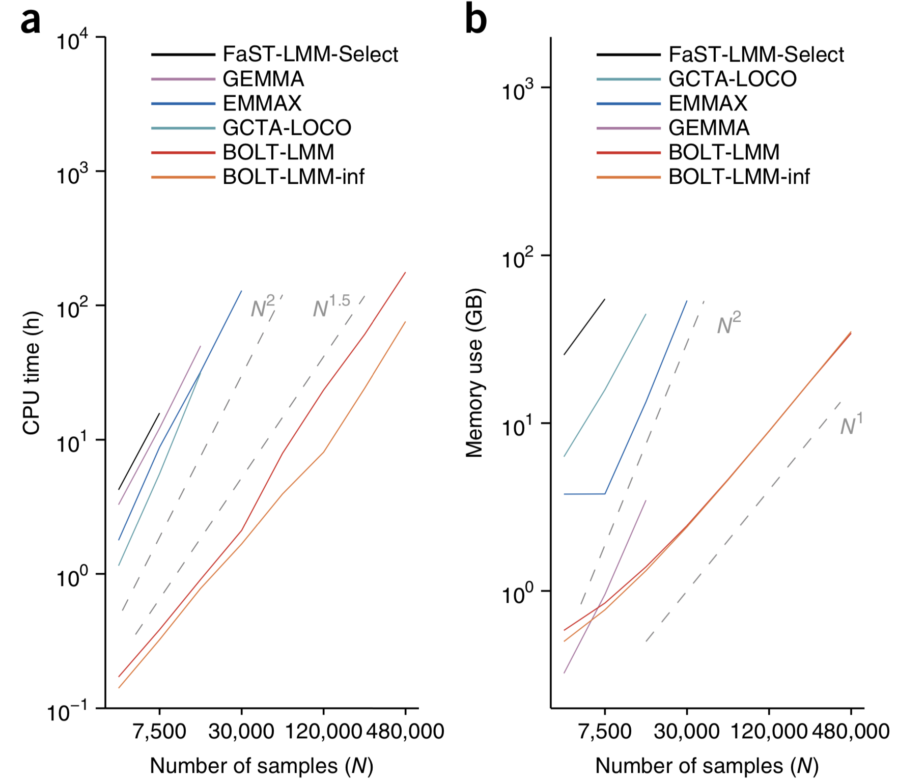
This is too slow for large samples (>20,000 individuals), i.e. exactly the sample sizes where one might expect to see most gains.
- BOLT-LMM (Loh et al., 2015), \(O(PN)\) https://data.broadinstitute.org/alkesgroup/BOLT-LMM/?
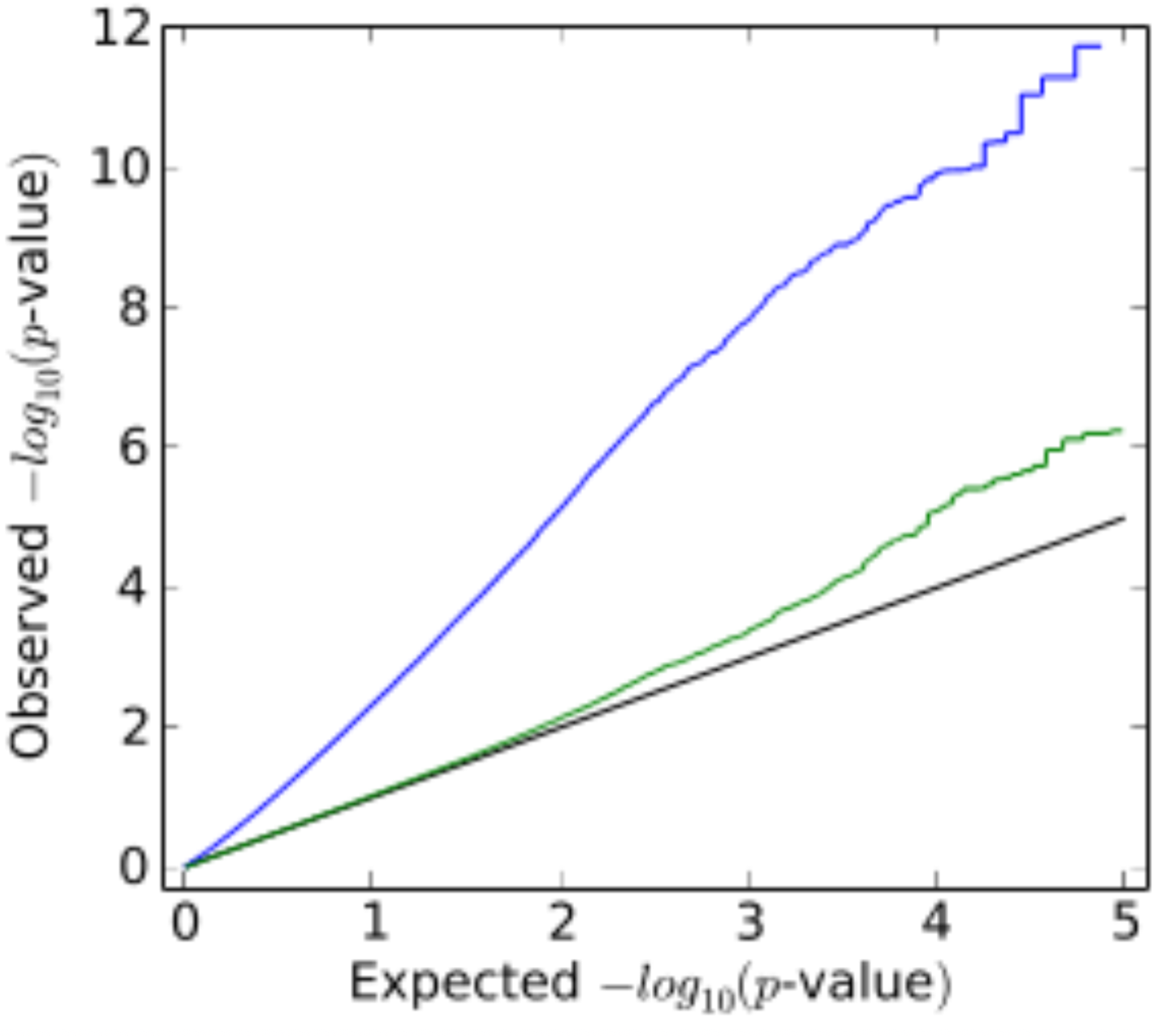
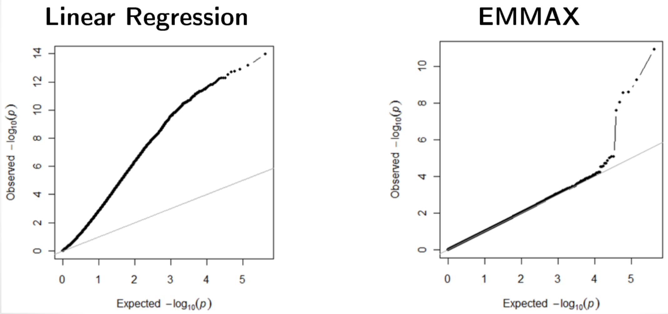
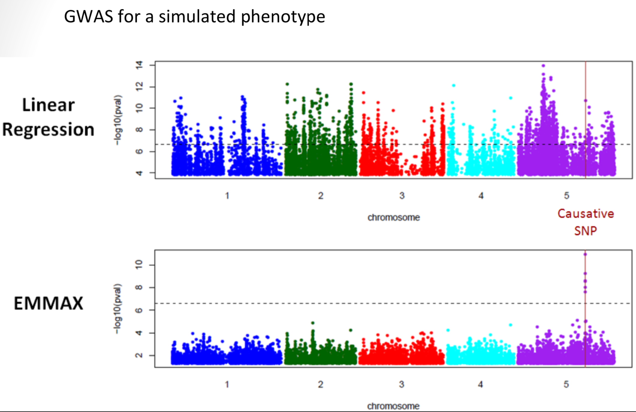
LMM reduce the test statistic inflation (Figure 11).
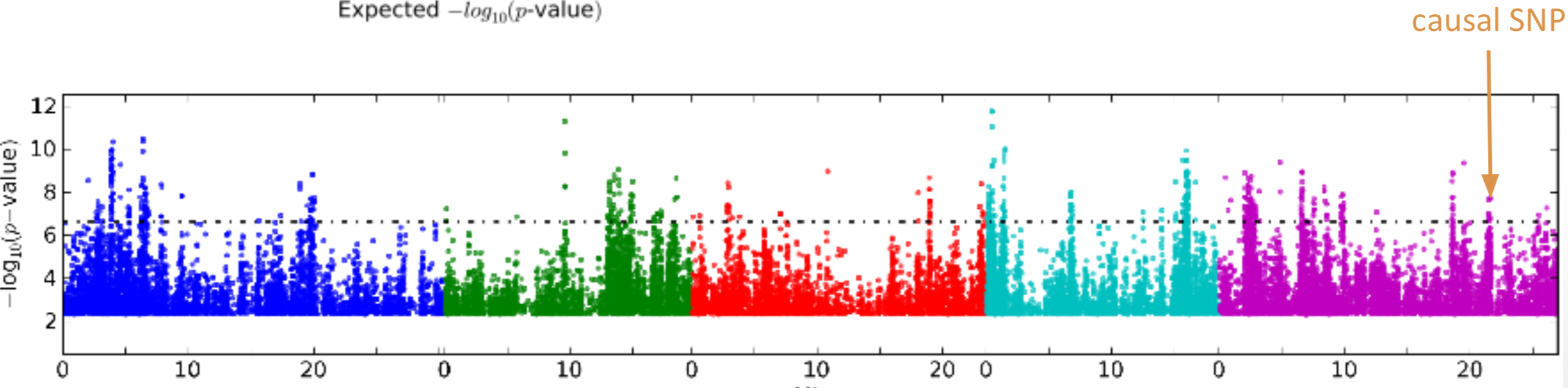
LMM also reduce false positives. Figure 12.
Advanced Mixed Models
The mixed-model performs pretty well, but GWAS power remain limited and need to be improved:
Multi Locus Mixed Model (MLMM),
- Single SNP tests are wrong model for polygenic traits
- Increase in power compared to single locus models
- Detection of new associations in published datasets
- Identification of particular cases of (synthetic associations) and/or allelic heterogeneity or linkage between causative polymorphisms.
- Combining correlated traits in a single model should thus increase detection power
Multi Trait Mixed Model (MTMM), Korte et al. (2012)
Traits are often correlated due to pleiotropy (shared genetics). When multiple phenotypes consists in a single trait measure in multiple environments, plasticity can be studies through the assessment of GxE interaction.
Caveats & Problems
Accounting for population structure does not alway work:
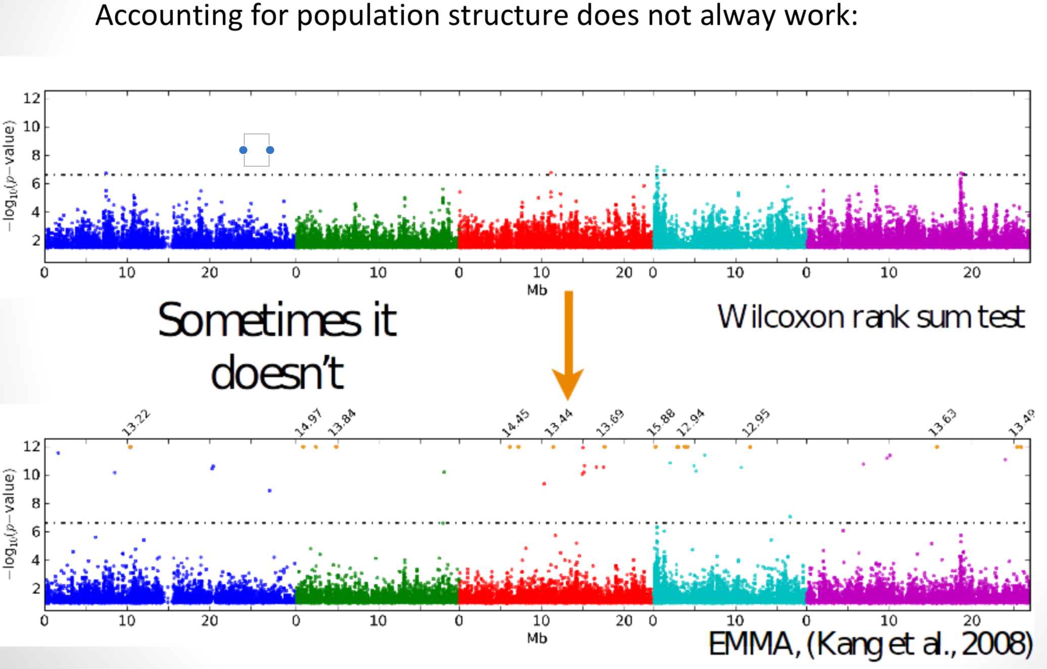
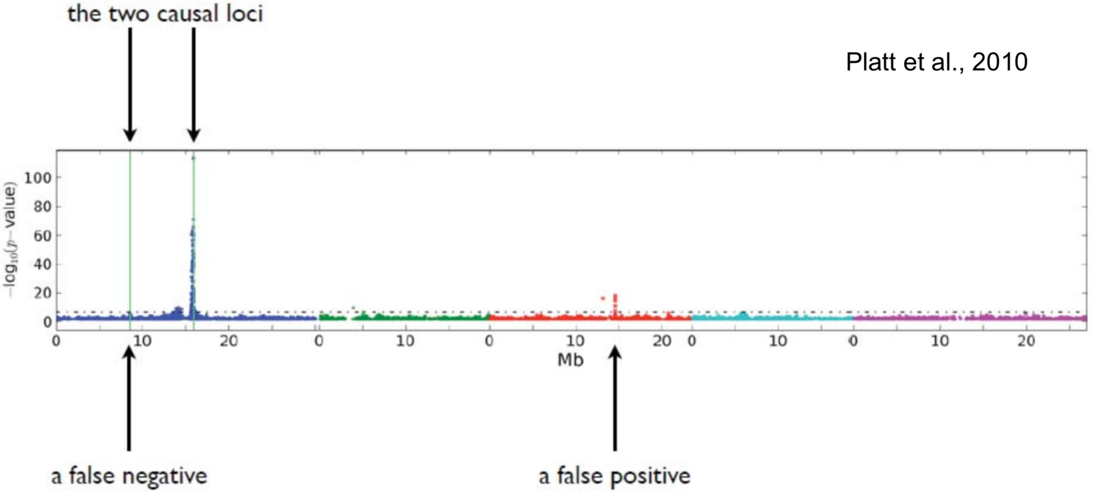
Sometimes it is difficult to decide which peaks are significant. One solution the the permutation of p-values.
Peaks are complex and make it difficult to pinpoint causative site
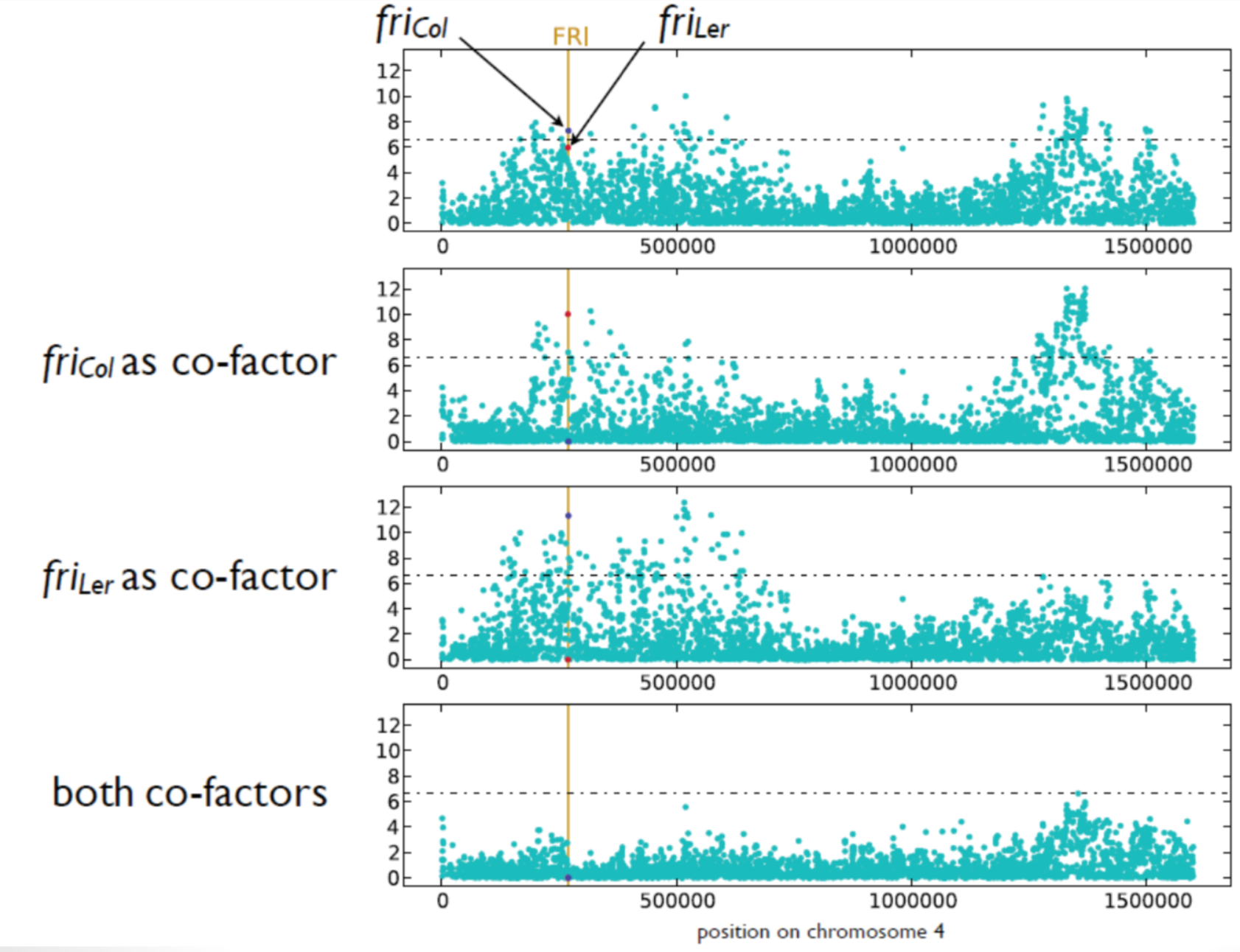
Condition under which GWAS will be positively misleading:
- More than one causal factor
- Epistasis
- Correlation between causal factors and unlinked non-causal markers
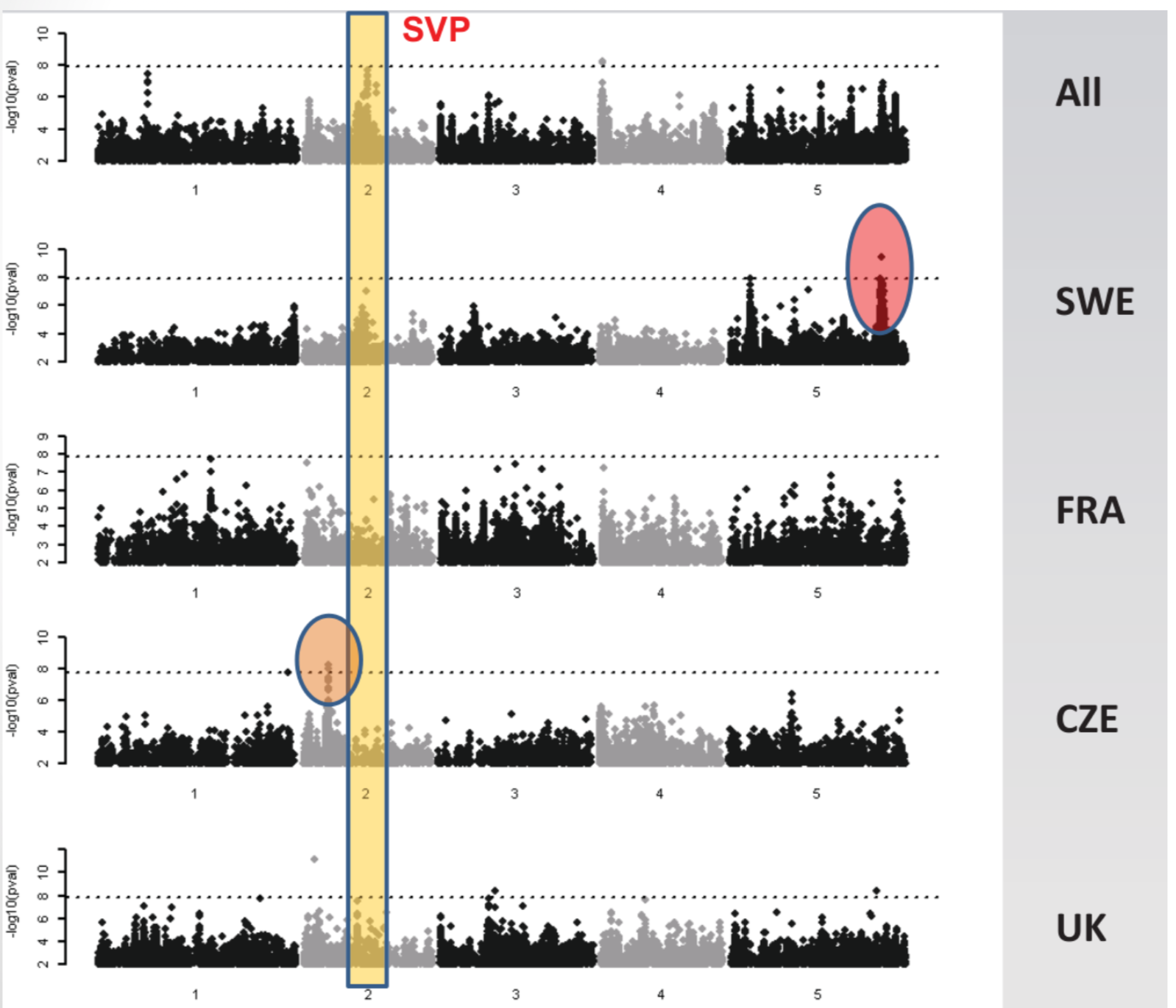
Different associations for different subsets (e.g., flowering time at 10°C).
- Highly heritable, easy to measure, polygenic trait
- 925 worldwide accessions
- Flowering time greatly varies in different populations
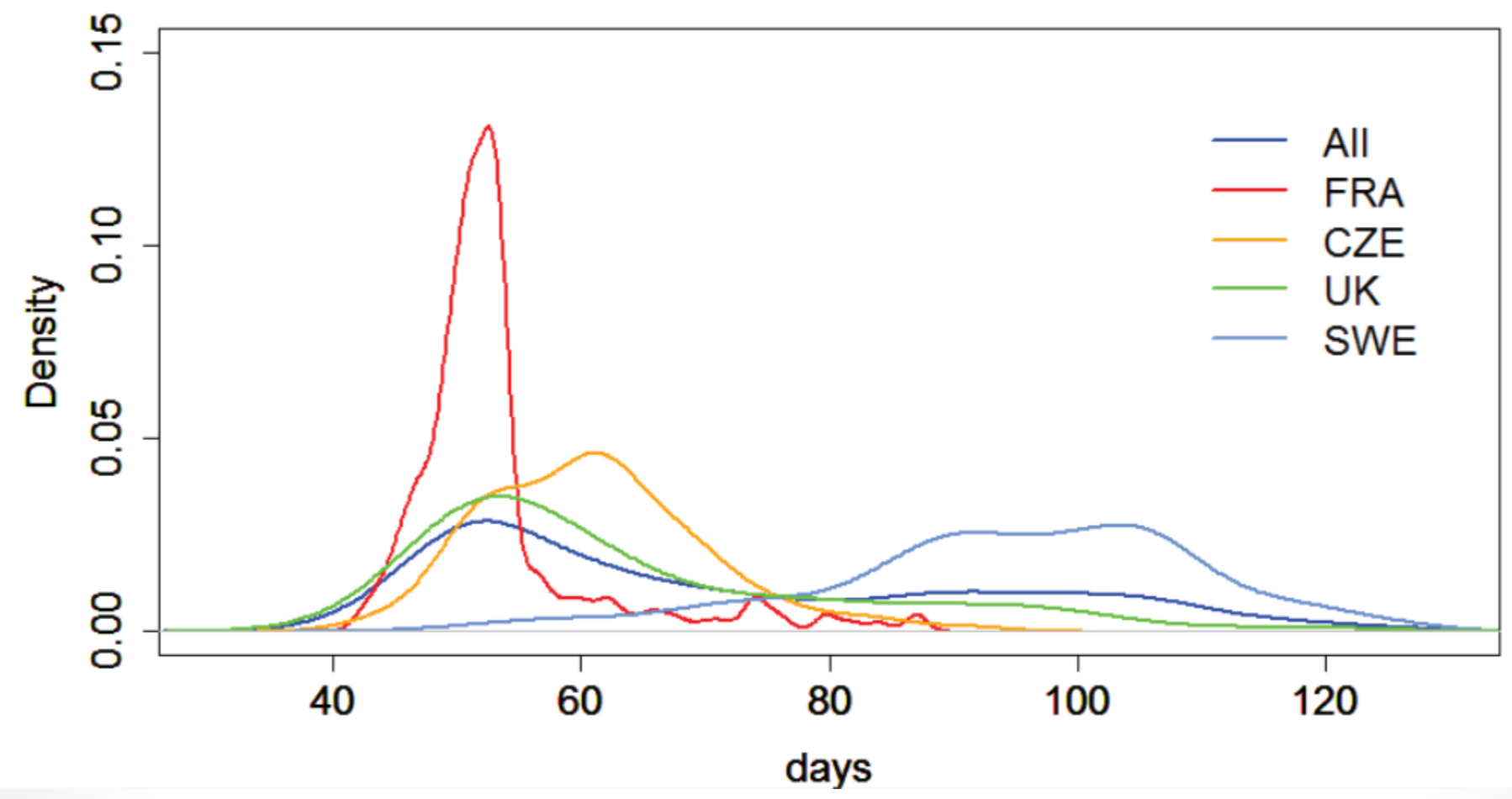
Significance and effect size differ dramatically in different subsets for the following reasons:
- False positives
- Effect depends on genetic background (Epistasis)
- Differences in allele frequency of the causal marker
- Artefact of LMM
Examples of GWAS in plant genetic resources
There are multiple examples where interesting genes GWAS were conducted in plant genetic resources to identify novel useful genetic variation after phenotypic evaluation.
In the following, two examples are shown.
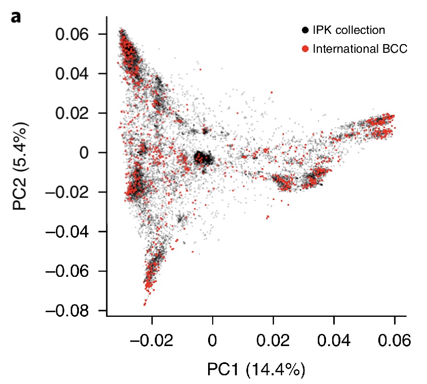
The barley collection in the German genebank at IPK is one of the largest barley collections worldwide. It has been genotyped using a method genotyping-by-sequencing (GBS), which is a reduced representation sequencing method because only about 2% of the genome is being sequenced. Using GBS, a total of 22,626 IPK genebank accessions were genotyped, of which 19,778 were domesticated barleys (Hordeum vulgare) and 1,140 wild barleys (Hordeum spontaneum) (Figure 13). Overall a, total of 171,263 SNPs were identified by GBS.
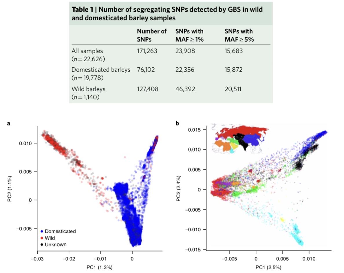
A population structure analysis with PCA of both wild and domesticated barley shows that a strong differentiation and within cultivated barley a strong differentiation between genetic regions (Figure 13 a and b). A comparison of a PCA of the complete IPK collection and the International Barley Core Collection further shows that the IBCC is a good representation of the total diversity of cultivated barley.
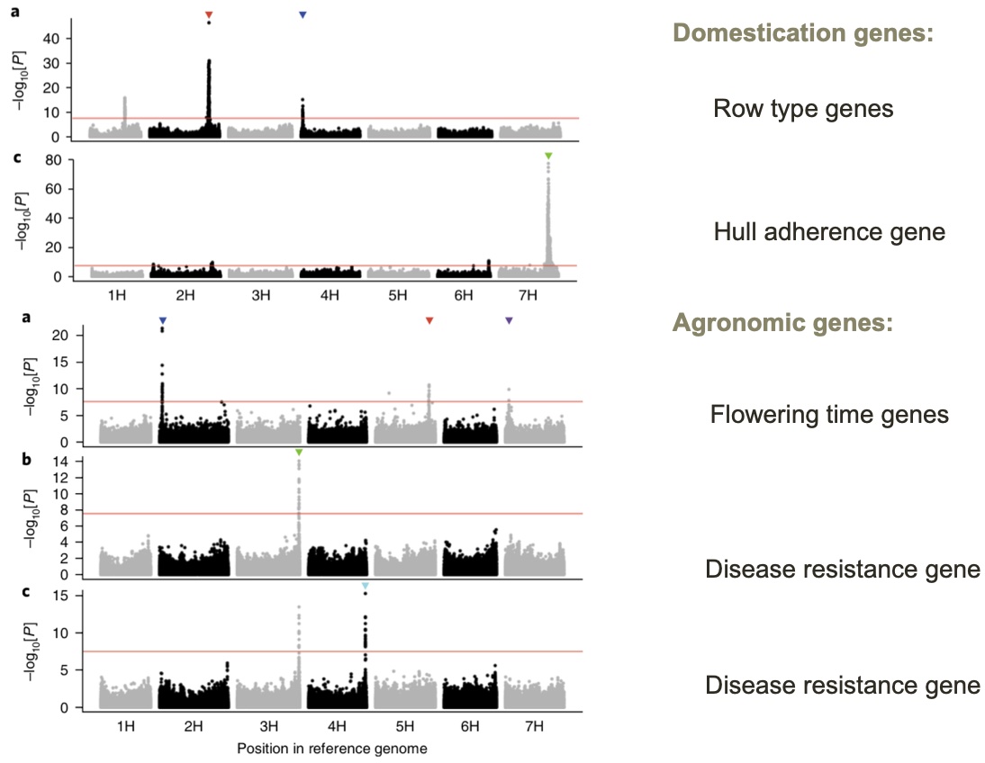
The IPCC was then used for large-scale GWAS analysis using a variety of domestication and improvement traits. Domestication traits were row type genes (2 or 6 row) and hull adherence, whereas agronomic traits included flowering time and disease resistance. The GWAS analyses detected several major QTL genes, of which some were known before, but also uncovered novel genes controlling these traits, which may be useful for further utilization in breeding (Figure 15).
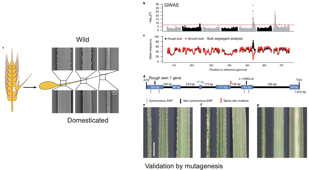
One example of such a gene is a gene for awn roughness, which is very different between wild and domesticated barley (Figure 16 a). Rough awns evolved allow grains to adhere to the fur of animals, for example, and therefore contribute to the geographic distribution (and ultimately, fitness) of wild barley. However, this trait is superfluous in domesticated barley, because seeds are not shattering anymore and the rough awns cause pain to the farmers during the harvest. A detailed analysis of the best hit in the GWAS analysis and in a related type of analysis called bulk segregant analysis identified the Rough awn 1 gene as causal gene for this trait. The causal mutation is a splice-site mutation, which changes the processed messenger RNA (mRNA) of this gene (Figure 16 b and c). This gene was validated as causal gene in a mutagenized barley population in which individuals with soft awns carried different mutations that also disrupted the funtion of the Rough awn 1 gene (Figure 16 d and e).
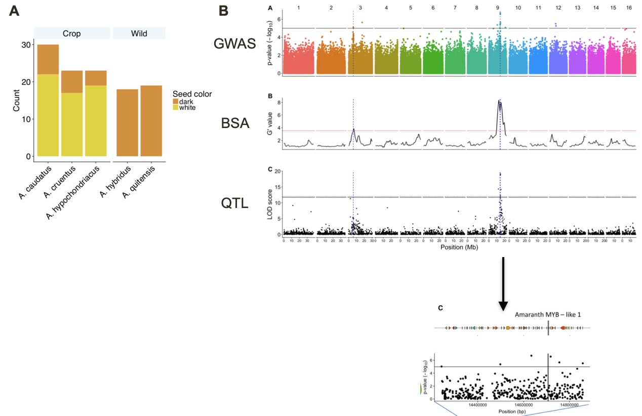
A similar study was carried out for an ancient crop of the Americas, amaranth. There are three types of grain amaranth (Amaranthus caudatus, A. cruentus and A. hypochondriacus) that were all domesticated from the same wild species, Amaranthus hybridus. A key domestication traits are white seeds in comparison to red seeds of wild amaranth. The whole genome resequencing of a set of wild and domesticated amaranths, and the subsequent GWAS, Bulk segregant analysis and QTL analysis of the trait revealed the same set of two genomic regions associated with the trait. The genomic region with the stronger statistical support harbors a so-called MYB-like transcription factor gene. Closely related genes (homologs) of this gene in other species were shown to be involved in controlling seed or fruit color by regulating the anthocyanin or betalain pathways. In the case of amaranth, further functional validation is required to test the hypothesis that the Amaranth MYB-like gene is a causal gene for seed color.
These examples (and many others in the scientific literature) show that GWAS of plant genetic resources is a powerful approach to identify many genes that may reveal the history of domestication or can be used in modern plant breeding programs using approaches like marker-assisted selection.
Key concepts
| \(\square\) Genome-wide association study (GWAS) | \(\square\) Genotype x Environment (GxE) interaction | \(\square\) Multiple testing problem |
| \(\square\) Confounding effect of population structure | \(\square\) Linear (mixed) model | \(\square\) Allelic heterogeneity |
Summary
- Genetic mapping with GWAS and related methods is a powerful approach to understand the genetics of phenotypic variation in plant genetic resources
- GWAS is based on the association between genotypic and phenotypic variation
- Population structure present in the analysed population may cause confounding and many false positive associations
- Multiple methods for GWAS are available.
- Methods based on linear mixed models are particular powerful because they can correct for population structure
- GWAS is challenging because epistatic interactions, allelic heterogeneity and GWAS on subsamples interfere with a simple interpretation of GWAS results
Further reading
- Cortes et al. (2021) - An accessible and timely review of GWAS in plants
Study questions
- What are the key differences between GWAS and QTL linkage methods for genetic mapping?
- What are the advantages and disadvantages of each of the two methods?
- Why doese population structure in a sample cause many false positive associations if it is not corrected by the model used for analysis?
- If there is a perfect correlation between a phenotypic trait of interest and population structure: Would GWAS be able to identify the causal gene, and would other methods be able to identify the gene controlling the trait?
- Why is allelic heterogeneity a problem in GWAS studies?
- Why is it useful and interesting to carry out GWAS in plant genetic resources?
- Which strategies can be used to further utilized significant trait-marker analysis from GWAS?