geneflow – Plant Genetic Resources (3502-470)

Motivation

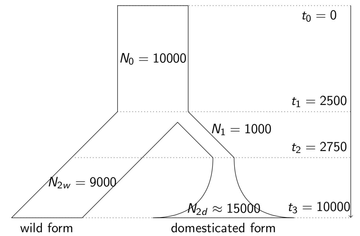
The analysis of gene flow is at the core of analysing and utilizing population genetic resources. So far, we have assumed a strictly bifurcating pattern of phylogenetic trees and in the analysis of genetic variation. For example, in studies of domestication, the most basic model assumes a single domestication event, after which the domesticated and wild relative evolve separately without any gene flow between them (Figure 1). However, both in natural settings as well in the context of agriculture and plant breeding, such a simple picture of the evolution of genetic variation is not appropriate. There are many instances of deviations from the bifurcating tree paradigm, in fact non-bifurcating trees often seems to be the norm rather than the exception.´ The most important processes that complicate a simple analysis of genetic variation are

Gene flow between populations and species
Reticulate evolution and hybridization of evolutionary lineages
Polyploidization of plant species.

We will discuss each of the following processes in the context of plant genetic resources and plant breeding.

Figure 1: A standard model of a single domestication. After domestication, the new crop species passes through a bottleneck phase before growing exponentially.

What is gene flow?

Gene flow is defined as the proportion of newly immigrant alleles of genes that move into a given population. The process depends on gene dispersal by migrations of individuals or their reproductive units (e.g., seeds or pollen), and the successful establishment of the dispersed alleles in the population. Different populations maintain a connectivity only by gene flow, and without it, populations diverge and may ultimately become different species. The extent of gene flow depends on the mode of reproduction and the mobility of individuals or their propagules. In wild species, gene flow also depends on the particular life style of a species, as well as on ecological conditions. In crop plants, the gene flow between wild crops, or GMO crops also depends on the patterns of crop cultivation (i.e., the human factor) or the presence of distinct breeding populations and the extent of exchange between breeding programs.

Why is it important to study gene flow?

In the context of plant genetic resources and plant breeding, the study of gene flow is important for several reasons. Studies on the history of a given crop species by analysing patterns of phenotypic and genetic variation should be based on models of evolution with migration. It provides a perspective on the ability and technical challengs for introgressing exotic germ plasm from genetic resources into modern breeding populations. The contamination of wild relatives of crops with genes from crops is determined by the extent of gene flow. The contamination of non-genetically engineered varieties with genes from genetically engineered varieties can be studied and modeled. The mobility of pollen and the rate of outcrossing vs. inbreeding determines the particular breeding method used for a crop species.

Processes affecting gene flow

The different biological characteristics of wild and crop plant determine the propensity for gene flow. A summary of processes affecting gene flow is given in Table Table 1.

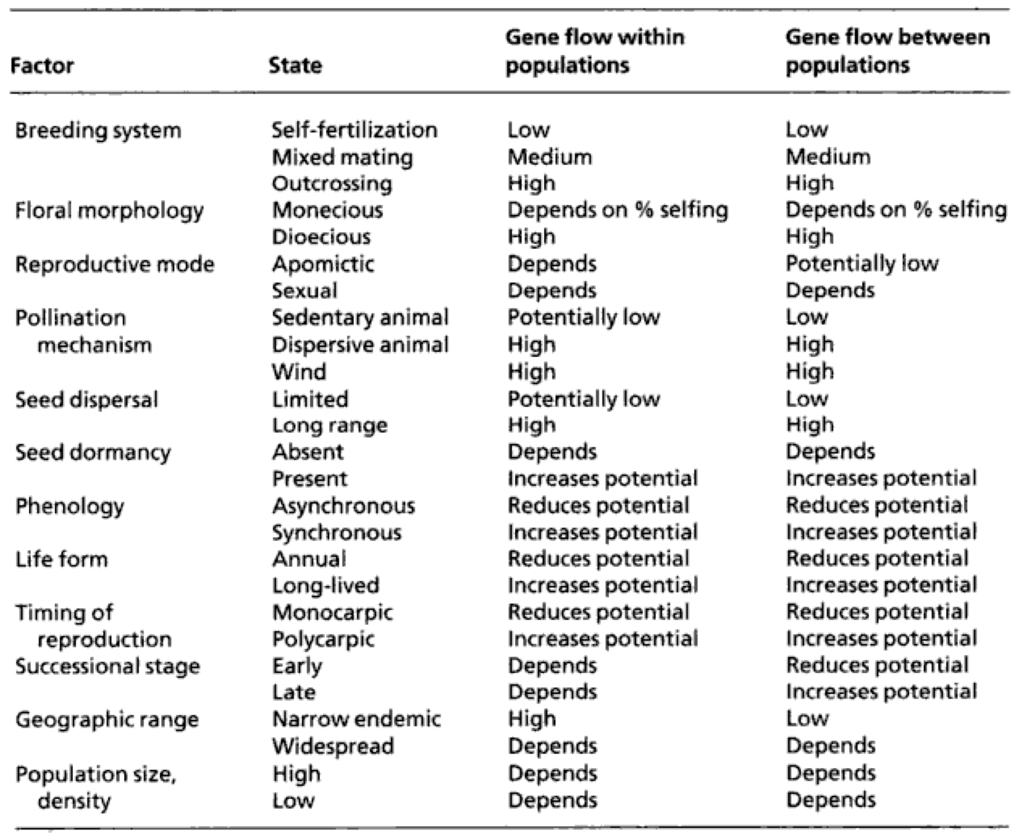
Table 1: Characteristics of plant species, which influence gene flow within and between populations. Source: Lowe et al. (2004)

The actual extent of gene flow is then determined by the combination of all biological characteristics present in a species. Some of these characteristics will be discussed in the following.

Sexual versus asexual reproduction

In sexual reproduction, two parents mate to form a zygote that contains genetic material from both parents. In contrast, in asexual reproduction, the resulting individuals are genetically identical (with the exception of new mutations) to the individual from which the originated by vegetative reproduction (e.g., runners, stolons, rhizomes, tissue fragments) or asexual modes of egg or seed production like, for example, apomixis (Wikipedia). In a sexual mode of reproduction, a new allele has to successfully introgress into a genome and into a population, whereas in the case of asexual reproduction, a new allele is introgressed only into a population, where it coexists with individuals that carry other alleles at the same locus.

The introgression of a new allele into a genome is only successful if the allele does not reduce the fitness of an individual. Fitness reduction can occur by the nature of the allele itself (i.e., a particular variant of an enzyme), but also by epistatic and pleiotropic interactions of the allele. The successful introgression of an allele into a population requires that the new allele does not reduce the fitness of the individuals carrying it in a given environment.

Self-fertilization versus outcrossing

Self-fertilizing species do not require that a pollen donor is present to successfully fertilize a flower.

Quite frequently, self-fertilization occurs before flowers are open (cleistogamy), and when pollen grains from other individuals reach the pistil of a self-fertilized flower, there may be no unfertilized egg cells left.

In contrast, outcrossing species depend on pollen from other individuals for a successful fertilization.

As a consequence, outcrossing species are expected to have much higher rates of gene flow because they are open to fertilization by immigrant pollen that may have dispersed across large geographic distances by wind or by animals.

Methods of dispersal

The methods of dispersal have a strong effect on the rate of gene flow. Several categories are to be considered:

Wind versus animal pollination
Size and robustness of pollen
Size and robustness of seeds
Wind, animal or unaided dispersal of fertilized seeds

Each characteristic that leads to a higher geographic dispersal ultimately will increase the rates of gene flow between populations.

Extrinsic factors

Everything else equal, the rate of gene flow depends also on extrinsic factors. They include:

The physical environment
Environmental selection factors
Abiotic and biotic environment

The physical environment can be described by physical barriers such as mountain ranges or large bodies of water (large lakes or oceans). They represent boundaries that suppress gene flow between populations.

Environmental selection factors include factors that affect the survival and the fecundity of a species. In plants, an important factor is flowering time. Strong environmental gradients may lead to different flowering times at geographically close populations. Asynchronous flowering then prevents gene flow even though dispersal between populations occur. If differentially adapted genotypes are dispersed into a single population, asynchronous flowering may prevent cross-pollination within a population.

The abiotic and biotic environment also acts as a selective agent. If favorable alleles are introgressed into a particular population, the rate of gene flow may be increased rapidly by selection. One example are new resistance alleles against pathogens, which may rapidly increase in frequency by natural selection. On the other hand, if everything else is equal, the particular abiotic and biotic environment may cause different rates of gene flow, in regions with different average strengths of wind (abiotic environment) or the presence or absence of pollinators or seed-dispersing animals (biotic environment).

In conclusion, rates of gene flow are determined by intrinsic and extrinsic factors. Estimates of gene flow rates need to account for both.

Lineage sorting mimicks gene flow

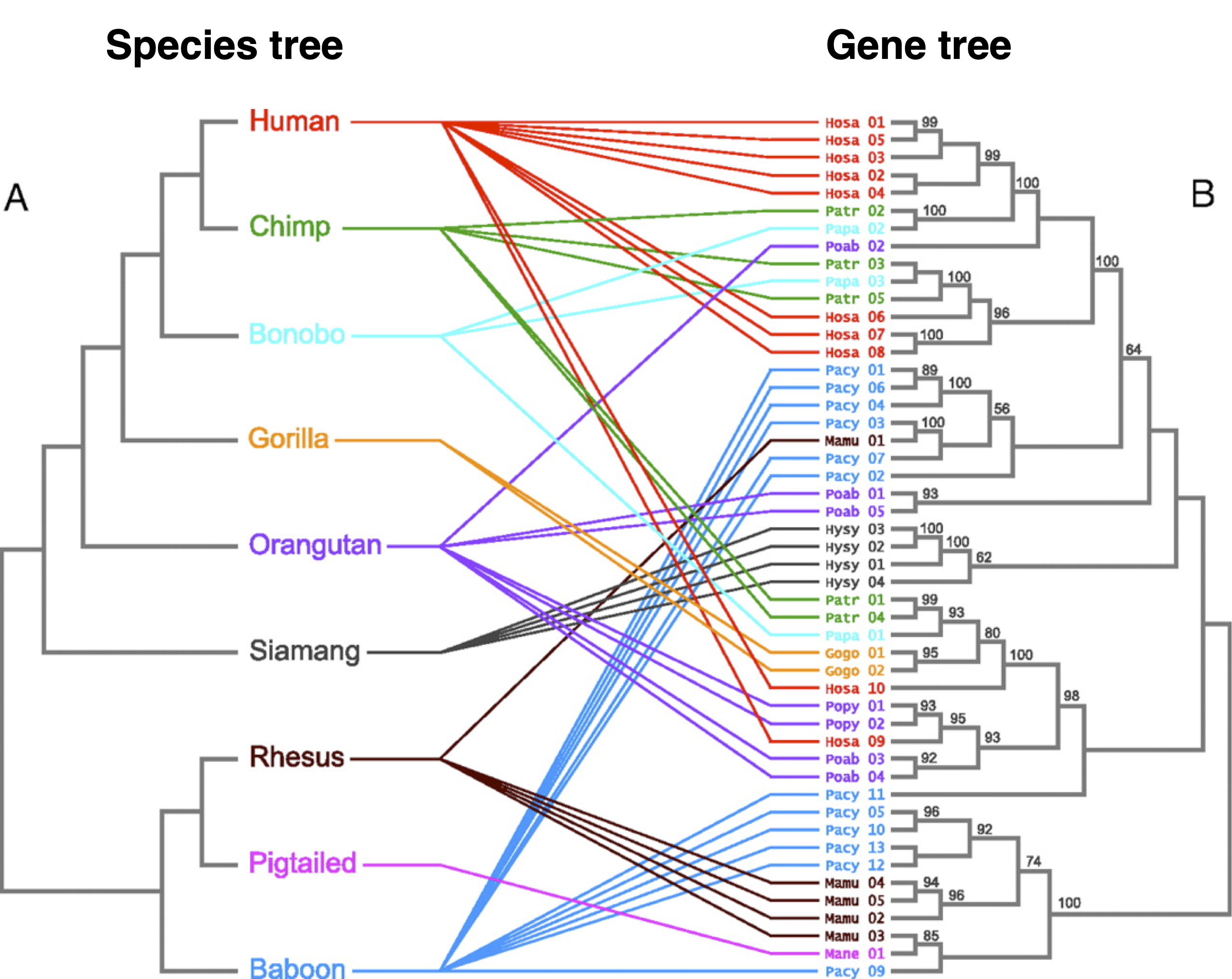
It is commonly assumed that the phylogenetic tree derived from an individual gene, the gene tree, resembles the species tree, which is the phylogenetic tree resembling the evolutionary relationships of the species. However, a gene tree and a species tree may actually differ significantly, for several reasons. Therefore, in order to reconstruct the species tree, it is necessary to look at many gene trees and calculate some kind of an average gene tree that may represent a species tree.

An illustrative example of a divergence between a species and a gene tree is shown in Figure 2. Due to the complex domestication history and/or polyploid nature of crop plants, the situation is often much more complex. For rice, for example, see the study by Cranston et al. (2009).

Figure 2: Comparison of a species tree with a gene tree in primates. On the left side there is the species tree of primate species, which represents the scientific consensus about the evolutionary relationship of primates. On the right side is the phylogenetic tree of a single gene, which plays a role in the immune response to pathogens. The tree contains several alleles from each species. This gene tree is extremely different from the species tree. Source: Loisel et al. (2006)

One important reason why a gene tree may differ from a species tree is lineage sorting. Imagine an ancestral population that splits into two evolutionary lines. If a polymorphism that is present in the ancestral population sorts itself in different ways among the descendant species, it is called lineage sorting. If both descendant species receive both alleles, a shared ancestral polymorphism is observed in both species. If an allele is lost in one of the two lineages (for example by genetic drift), a phylogenetic patterns arises at the locus that is confusing or inconsistent with the species tree. This process is called lineage sorting because different alleles ‘survive’ into the present in different lineages. Sometimes only an ancestral allele has been lost in one lineage, but not in the other, which is still polymorphic. In this case, the gene tree does not represent the species tree because the resulting phylogeny is a paraphyletic rather than a monophyletic tree. This process is called incomplete lineage sorting (Figure 3 B).

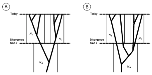
Figure 3: Complete and incomplete lineage sorting after a single ancestral population split into two new populations. Source: Arbogast et al. (2002)

Incomplete lineage sorting interferes with the analysis of gene flow because it produces a pattern that is similar to recent migration between populations.

Therefore, shared ancestral polymorphisms between, for example, a crop and its wild ancestor may either result from recent gene flow or represent incomplete lineage sorting.

Reticulate evolution

If two evolutionary lineages merge together, and subsequently evolve as a single evolutionary lineage, it is called reticulate evolution. There are numerous examples of reticulate evolution in the plant world. They include:

The merger of plants with cyanobacteria that evolve into chloroplasts.
The merger of ancestors of modern eukaryotic cells with bacteria to form mitochondria.
The hybridization of two plant species that merge into a single new, hybrid and allopolyploid plant species.

Hybridization

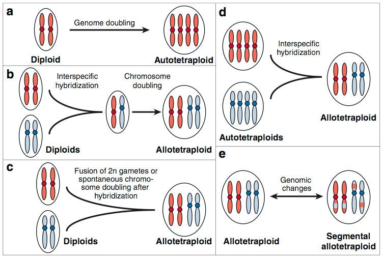
Hybridization is the merger of two or more genomes into a new, polyploid genome (Figure 4). If genomes originate from the same species, the process is called autopolyploidization, if the genomes originated from different species, it is called allopolyploidization. Although both types of polyploidization are hybridization processes, the term is usually used if the genomes originate from two different species. In plant evolution, hybridization occurred extremely frequently, and nearly each plant species has experienced a polyploidization event.

Figure 4: Illustration of auto- and allopolyploids. For simplicity, only one pair of homologous chromosomes (either in red or blue) is shown in a diploid. (a) Formation of an autotetraploid by doubling a basic set of chromosomes. A triploid (not shown) can be formed by hybridization between a diploid and an autotetraploid. (b) Formation of an allotetraploid by interspecific hybridization followed by chromosome doubling. (c) Formation of an allopolyploid by fusion of unreduced gametes in two diploid species. (d) Formation of an allotetraploid by interspecific hybridization between two autotetraploid species. (e) An allotetraploid (left) may become a segmental allotetraploid (right) if homoeologous chromosomes contain some homologous chromosomal segments. Source: Chen (2007)

Examples of crops with a history of polyploidization are:

Autopolyploidization: Potato
Allopolyploidization: Durum wheat, emmer wheat, bread wheat, peanut

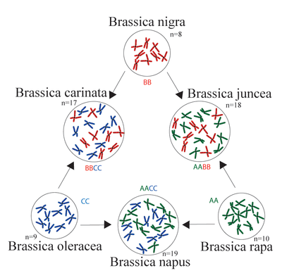
A very well characterized example of the polyploidization is the triangle of U (Figure 5), which explains the origin of three different tetraploid Brassica crops from different diploid ancestors.

Figure 5: The triangle of U, a model to explain the origin of Brassica crops. Source: Wikicommons.

Domestication history of wheat

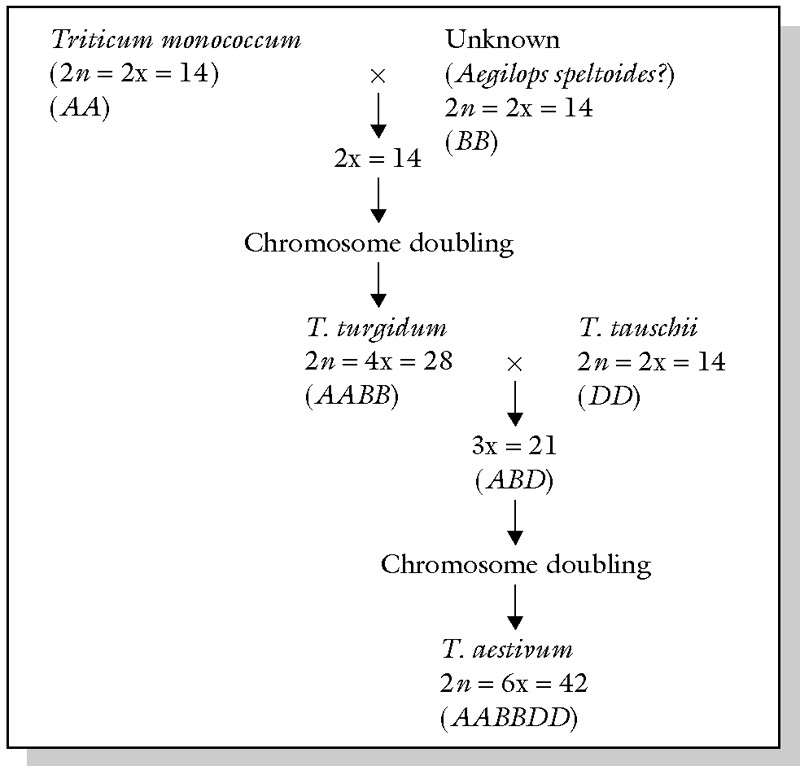
Many crop species are polyploids that arose recently by hybridization. The most important polyploid species is wheat, which has a complex history of hybridization and polyploidization. Figure 6 shows a model of bread wheat domestication. It should be noted that some research treat wheat as a single, large genus Triticum sensu lato, whereas others consider them to consist of two separate genera, Triticum and Aegilops. A summary of the different classification systems can be found at http://www.k-state.edu/wgrc/Taxonomy/taxintro.html.

The bread wheat Triticum aestivum is a hexaploid ($2n=6x=42$, AABBDD) and was probably domesticated in two steps Andersson and de Vicente (2010):

Hybridization of a diploid A-genome and a diploid B-genome donor. The A donor was likely the wild T. urartu Thumanjan ex Gandilyan. The B genome originated from Aegilops sect Sitopsis (Jaub & Spach) Zhuk., possibly from Ae. speltoides (or one of its ancestors because the B genome in this species most closely resembles that of bread wheat. Hybridization between these two diploid species led to the evolution of the tetraploid wheat progenitor wild emmer (T. turgidum subsp. dicoccoides (Körn. /ex./Asch & Graebn.) Thell.)
The second hybridization event occurred between domesticated tetraploid emmer (T. turgidum subsp. dicoccum), which was the donor of the AB genome, and diploid Ae. tauschii, the donor of the D genome.

Figure 6: A model of bread wheat domestication by hybridization. Source: Acquaah (2009)

Important aspects of wheat domestication are:

the hybridization of species from different genera.
the creation of several independent wheat species, such as emmer wheat (diploid), durum wheat (tetraploid) and bread wheat (hexaploid)
the ability to utilize the ancestors of bread wheat for introgression of genetic variation. Hybrids can be relatively easily obtained with species that share a common (A,B or D) genome.
the ability to re-synthesize neopolyploids from different individuals of the same of closely related parental species

In summary, wheat should be seen as a complex genetic and genomic system, which is highly flexible and which demonstrates an important feature of hybridization and polyploidization. Hybridization often leads to the expression of transgressive characters, which are more extreme characters than of their parents.@tbl-polyploidfeatures). Polyploid hybrids are frequently found in very different and extreme environments than their parental species. Polyploid individuals are frequently more robust and larger than their parental taxa.

::::: {.content-hidden .comment ::: {#tbl-polyploidfeatures}

Characteristics of polyploid plants. Source: Lowe et al. (2004).

::: :::::

Frequent characteristics of polyploids

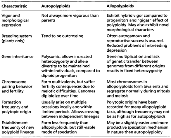
Polyploidy is very common in the plant kingdom because it frequently provides evolutionary advantages (i.e., a higher evolutionary fitness). Many crop plants are fairly recently evolved polyploids. In addition there are some critical differences between autopolyploids and allopolyploids, such as wheat or quinoa.

Vigor and Morphological Expression

Autopolyploids are not always more vigorous than their diploid parents. In contrast, allopolyploids often exhibit hybrid vigor due to the combination of genomes from different progenitors. This is sometimes referred to as the “gigas” effect, reflecting the increased size or robustness in plant traits. Additionally, allopolyploids may display novel morphological characteristics not seen in their parents.

Breeding System (Plants Only)

In terms of breeding systems, autopolyploids tend to be outcrossing, which promotes genetic diversity through mating between different individuals. On the other hand, allopolyploids are often autogamous (self-fertilizing), which ensures reproductive success even in isolated environments. This also leads to reduced problems of inbreeding depression due to their fixed heterozygosity.

Gene Inheritance

Autopolyploids typically exhibit polysomic inheritance, which allows for increased heterozygosity and the maintenance of greater allele diversity within individuals, compared to their diploid ancestors. Allopolyploids, however, show gene multiplication with limited genetic exchange between distinct genomes, leading to fixed heterozygosity—a stable retention of genetic differences between the contributing genomes.

Chromosome Pairing Behavior and Fertility

In autopolyploids, chromosomes often form multivalents during meiosis, which can lead to fertility issues due to irregular chromosome segregation. However, genomes tend to diploidize over time, reducing these issues. Conversely, in allopolyploids, chromosomes typically pair as bivalents and segregate normally during both mitosis and meiosis, supporting higher fertility and genetic stability.

Formation Frequency and Polytypic Origin

Autopolyploids tend to arise repeatedly, often within local populations and during short time frames. This repeated formation enables crossing between independently formed lineages. Allopolyploids also have polytypic origins, and many taxa have recorded multiple independent formation events, though this may occur less frequently than in autopolyploids.

Establishment Frequency of New Polyploid Lineage

The establishment of new lineages occurs less frequently in autopolyploids than in allopolyploids, although autopolyploidy still provides a viable pathway for speciation. Allopolyploidy, by comparison, is slightly more common and effective as a speciation mechanism in nature.

Let me know if you’d like this formatted for teaching materials (e.g., slide notes or lecture handouts) or turned into a table in Markdown or LaTeX.

Methods for analysing gene flow and reticulate evolution

Considerations in the analysis of gene flow

There are two basic types of methods for analyzing gene flow.

Indirect methods characterize how genetic variation is distributed throughout current populations. This information is used to infer past and recent processes of gene flow between the populations. In indirect methods, only successfully established alleles are included. Unfortunately, other processes may lead to similar patterns of genetics variation, and it may be possible to differentiate between current patterns of gene flow from historical population colonization processes that are of little relevance for current patterns of gene flow in a given landscape.

Direct methods asses the transfer of genetic material in arrays of parents and offspring to calculate the rates of gene movement of gametes or other propagules. This method allows the estimation of gene dispersal. However, these methods do not allow to analyze the rate by which new alleles in a population are successfully established. The dispersal of GMO seeds and pollen is frequently studied with direct methods.

Both the direct (or observational or process-based) and the indirect (or pattern-based) methods for analysing gene flow have advantages and disadvantages that need to be considered in the design of a study.

Overall, indirect methods are more powerful than direct methods, for the following reasons:

Higher efficiency of molecular markers than of direct observations.: For various reasons, it is difficult to obtain a large sample size with observational studies (i.e., labelling experiments of pollen). High-marker densities provide more information.
Missing of rare, long-distance dispersal events.: Observational studies often miss long-distance, rare dispersal events that are frequently important for the introduction of new genetic variation into a population.
Observation of dispersal but not gene flow.: Observational methods often focus on analysing dispersal of gametes or seeds but do not take into account post-dispersal factors such as viability, sexual compatibility, gamete competition or selective embryo abortion. Neglecting these factors may lead to an overestimation of gene flow rates.
Focus on individuals rather than populations in process-based methods.: By selecting few or relatively few individuals, it is much more difficult to obtain population estimates of migration and gene flow than with pattern-based methods using genetic markers.

In the following, only indirect methods will be discussed.

Indirect methods often make numerous assumptions, which need to be considered in the design, analysis and interpretation of gene flow between populations. The most important assumptions are

Unrealistic models:: The $F_{ST}$ statistics as described below assumes an island model, where gene flow rates are estimated between islands. However, the estimates also reflect other evolutionary processes such as selection or historical population expansion, which violates population models.
Relative versus absolute estimates.: In most cases, only relative estimates of gene flow with respect to different gametes or zygotes are obtained. In some applications, it is important to obtain absolute estimates of gene flow, for example in estimates of gene escape from GMO plants or in the management of genetic resources. In both cases, individual events already have a profound effect.
Unrealistic population structure:: Frequently, unrealistic assumptions about the population structure are made that include randomly mating metapopulations of equal size, or a mutation-drift equilibrium within a population.
Complex parameters:: Indirect estimates of gene flow rates estimate complex parameters that, for example, also include the effects of selection and genetic drift. It is often difficult to disentangle the different parameters.

Analysis of clones and inbreeding

The geographic dispersion of clones and genes can be easily studied by using any genetic fingerprinting technique using a sufficient number of markers. It is expected that all clonal individuals (genet) are genetically identical and reveal the same fingerprint pattern. For this reason, a geographic analysis is relatively simple.

To analyse the extent of inbreeding, the $F_{IS}$ statistic can be used.¹ It is calculated as \[\begin{equation} \label{fis} F_{IS} = 1 - \frac{H_{obs}}{H_{exp}} \end{equation}\] with $H_{obs}$ as the observed heterozygosity (proportion of heterozygous loci) and $H_{exp}$ as the expected heterozygosity, which is calculated as from the allele frequencies under the assumption of a Hardy-Weinberg equilibrium.²

¹ For an overview of Wright’s $F$ statistics, see the script on population and quantitative genetics.

² For an overview of Wright’s $F$ statistics, see the script on population and quantitative genetics.

Phylogenetic approaches to analyse gene flow

There are numerous methods available for the analysis of gene flow and reticulate evolution using phylogenetic methods

The basic approach to detect gene flow in a gene is the following:

Construct a phylogenetic tree of a sample of individuals from different populations using a genome-wide set of markers or large number of genes (Species tree).
Compare an individual gene tree with the species tree-
Apply a statistical test to check whether the high stochastic variance of gene trees causes it to be significantly different from the species tree.

Different patterns of population structure and migration can be demonstrated by the expected trees in Figure 7. In the Figure, four scenarios are considered:

Trees from a single coalescent simulation
Split from an ancestral population $4N$ generations ago
Migration: 0.5 migrants per generation in each direction
Six alleles per generation were sampled

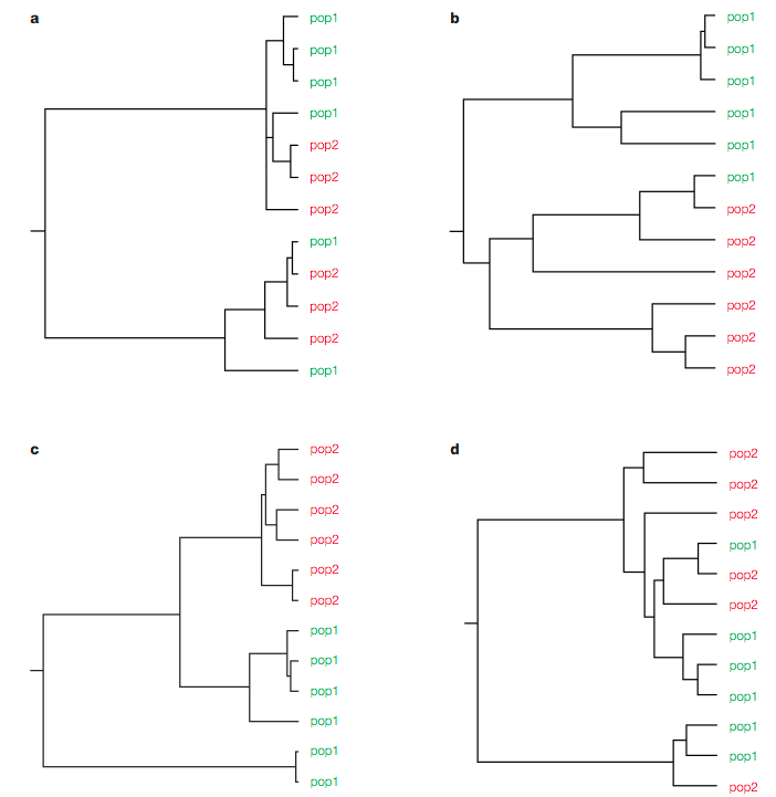
Figure 7: Four different outcomes of coalescent simulations with different levels of population structure and migration. Source: Hey and Machado (2003)

The simulated trees can represent four different scenarios:

Tree a: Strongly separated pop, recent gene flow
Tree b: Recently separated population, single gene flow event
Tree c: Separation of populations some time ago, no gene flow
Tree d: Both populations appear to be a single panmictic population.

The challenge is to find a statistical approach to test which of the scenarios is the real one.

One complication of phylogenetic approaches is the effect of recombination on gene genealogies. Recombination has the effect that different regions of the genome have different geenealogies (Figure 8)

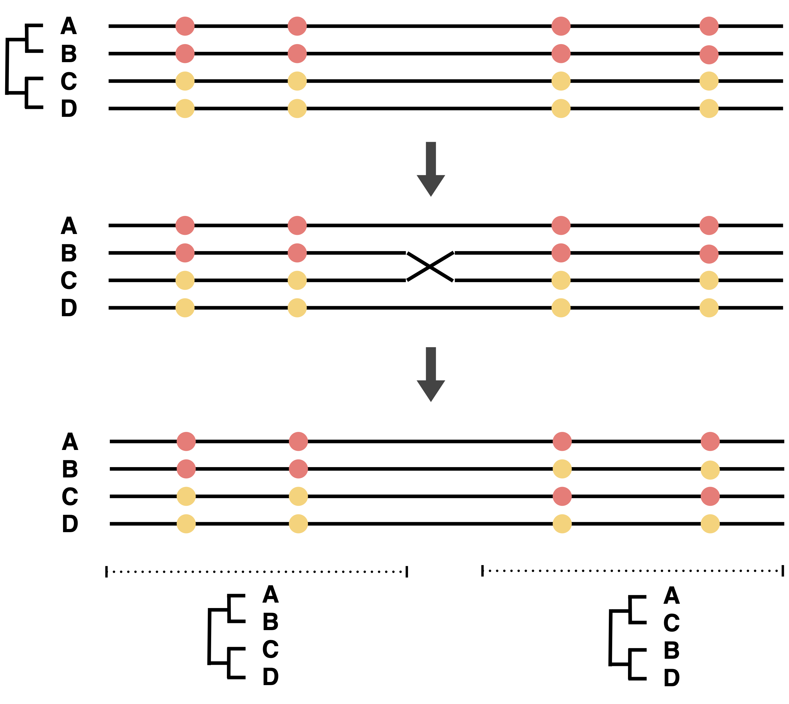
Figure 8: Effect of recombination on the gene genealogies of linked regions

In any comparison between an individual tree and the species tree, the effect of gene-specific stochastic effects plus the effect of recombination have to be accounted for.

A test of gene flow using a phylogenetic analysis is carried out with the following approach:

Sample multiple genes $\rightarrow$ ‘average’ gene tree $\approx$ species tree
Use maximum likelihood or Bayesian framework
Calculate probability that a given gene tree corresponds to the species tree $\rightarrow$ identify genes with gene flow

Phylogenetic networks

The phylogenetic trees were constructed without considering the effects of recombination. However, as shown in Figure 8, recombination in a genomic segment produces different genealogies for adjacent regions, which result in conflicting phylogenies for the whole regions. One way to represent such phylogenetic conflicts (i.e., sequence regions with recombination) is phylogenetic networks. Phylogenetic trees of genomic regions with recombination, hybridization or gene transfer can be represented as multifurcating trees or networks. They have the advantage that they do not ‘force’ data onto a simple bifurcating tree.

There are different types of networks:

Statistical parsimony networks
Split networks

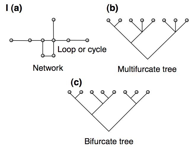
Networks can be used to evaluate the deviation of a given tree from a bifurcating tree. Examples of the different types of trees are shown in Figure 9.

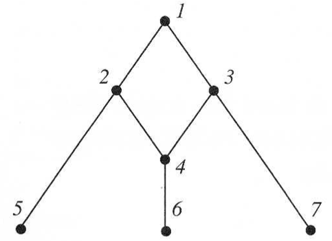
Figure 9: Types of phylogenetic trees and networks. Source:Posada and Crandall (2001)

A simple network is shown in Figure 10.

It can be interpreted as follows:

Taxa 5,6,7 are extant (current) taxa
Taxon 1 is common ancestor
Ancestors 2 and 3 interacted to create 4
Taxa 1,2,3,4 form a cycle

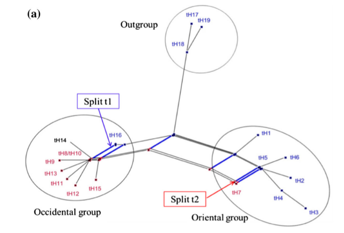
Figure 10: A simple network consisting of four nodes.

Split networks

A split is any edge in an unrooted phylogenetic tree that defines a partition of a set of taxa into two groups (bipartition) of distinct subsets.

Strictly bifurcating phylogenetic trees contain only splits that are compatible, whereas networks contain incompatible splits. Such networks are called split networks.

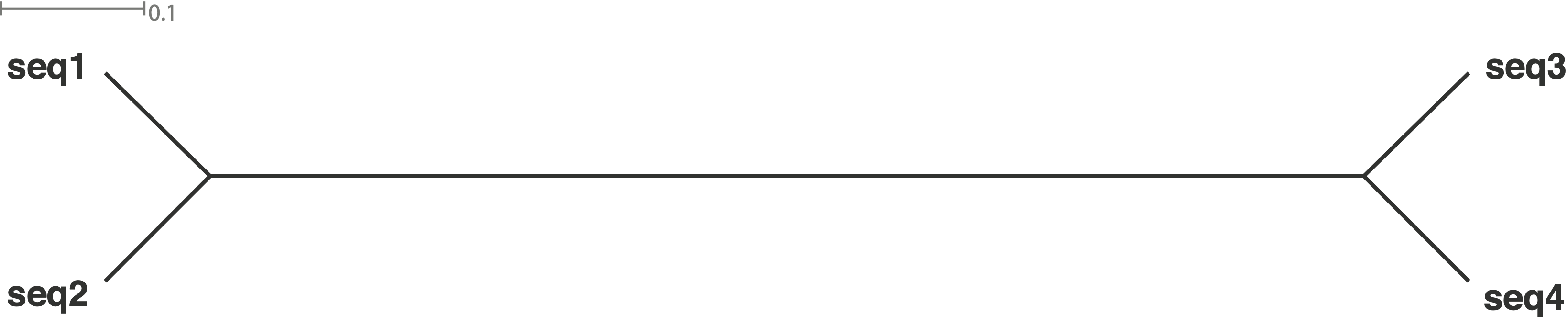
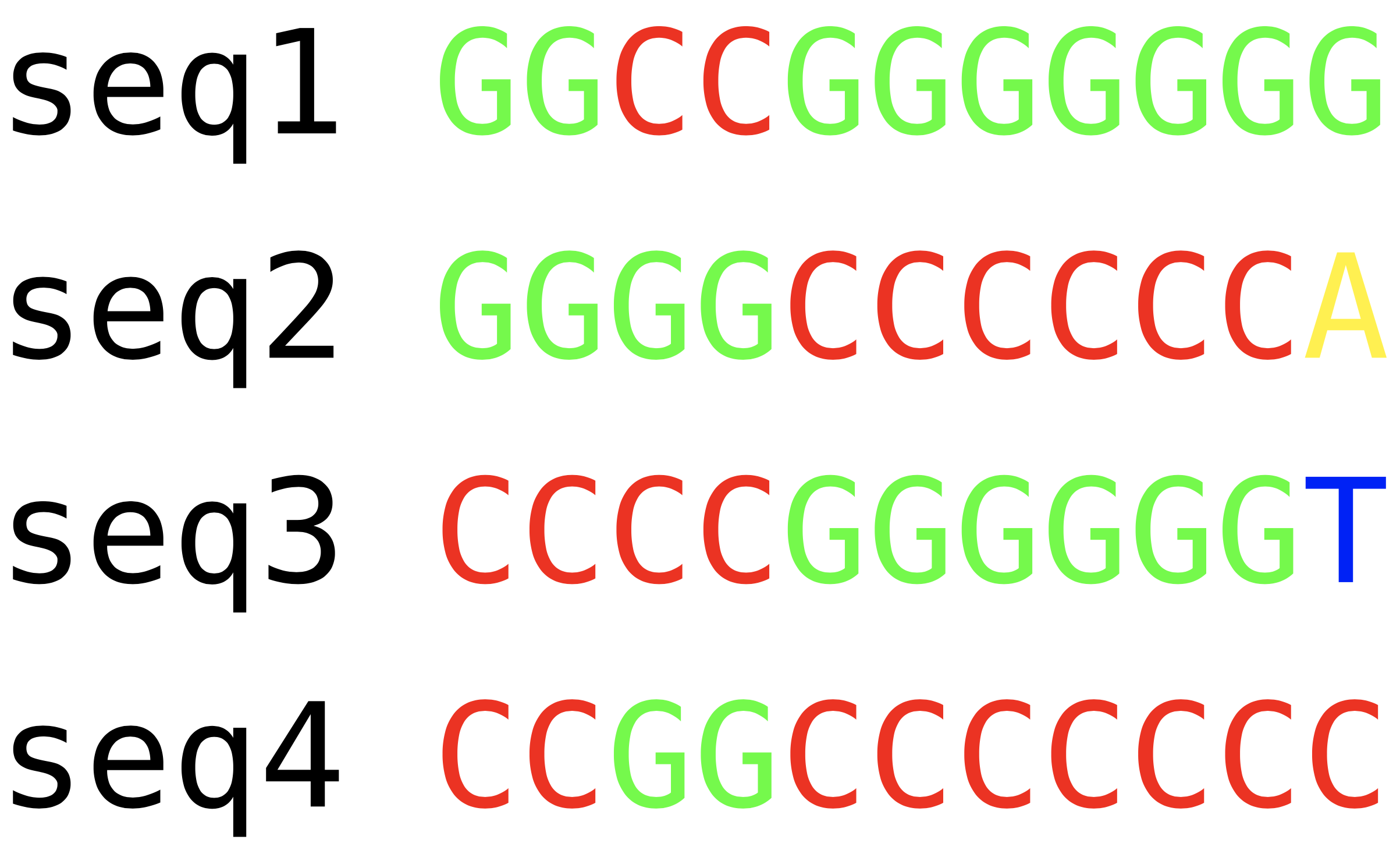
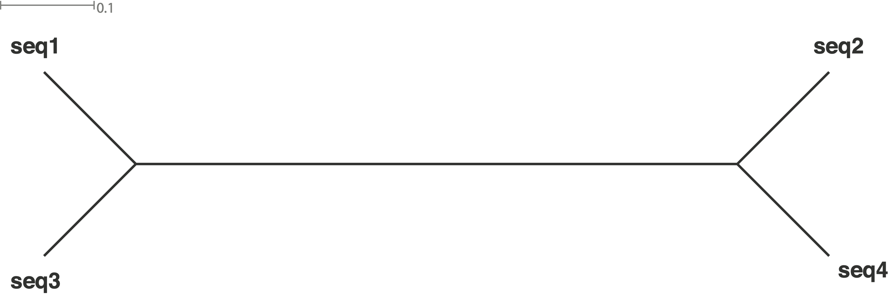
The following #fig-seqaln1 shows a sequence alignment without any conflicting signals. the resulting tree is shown below in Figure 14.

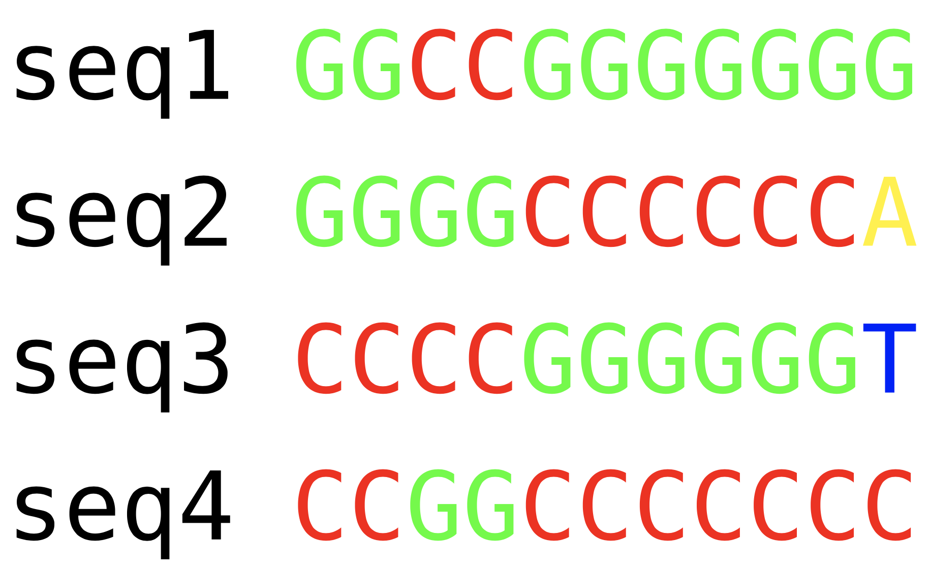
The resulting phylogenetic tree is shown below in Figure 14.

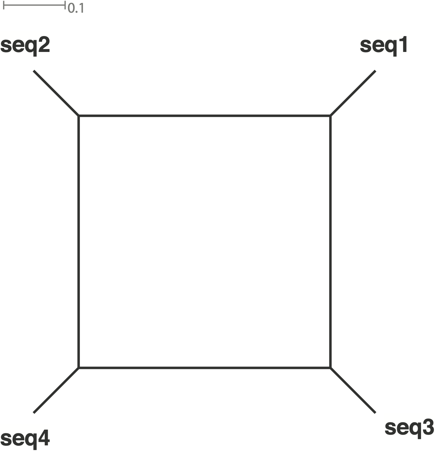
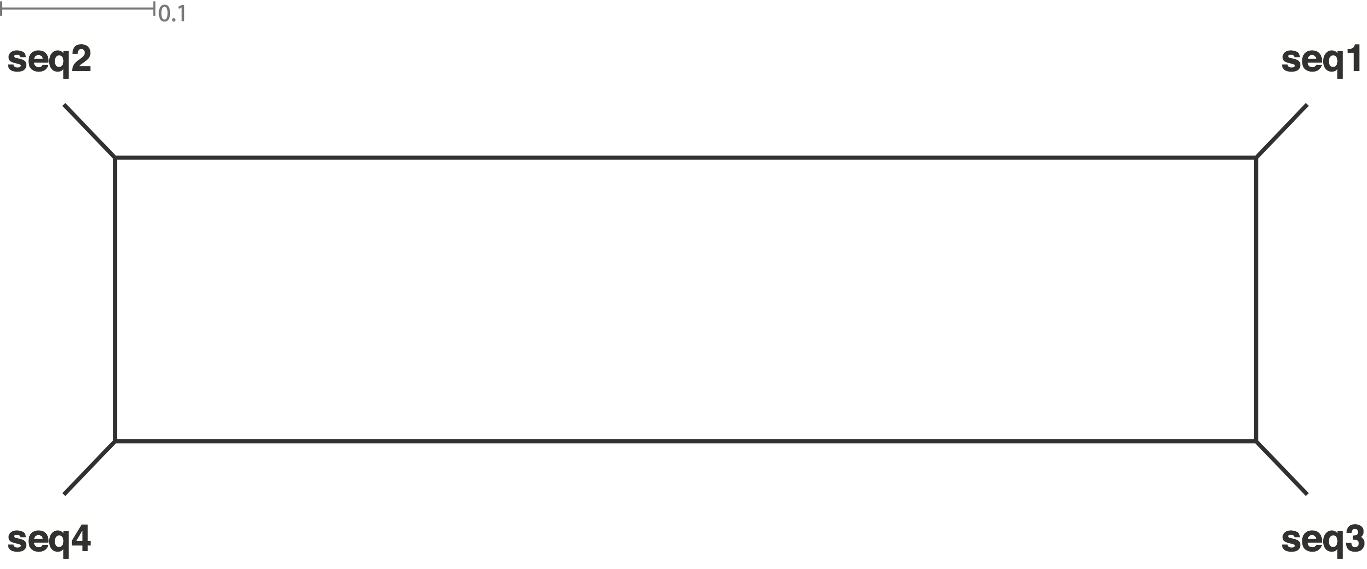
Figure 12: A strictly bifurcating tree. label:fig:net1

If there are conflicting signals, several splits of the same accessions are possible and equally likely, as shown in the tree.

An alignment with phylogenetically conflicting signals is shown in Figure 13.

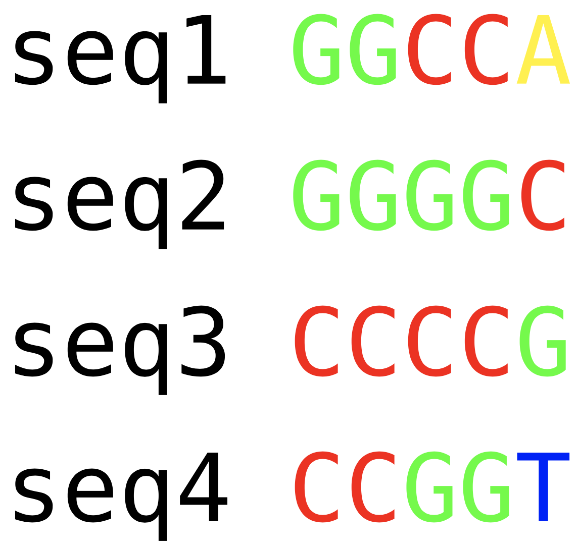
And the resulting network is shon in #fig-net2.

Here is a sequence alignment with different proportions of conflicting signals.

The relative proportion of conflicting signals is expressed by the length of the splits.

The corresponding strictly bifurcating Neighbor-Joining tree of the last example is then

To summarize, split networks show the extent of conflicting phylogenetic information. For this reason, they are suitable for the analysis of introgression, gene flow and reticulate evolution.

Applications and examples

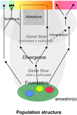
The domestication of plants is arguably one of the most complex processes in the history of population because many different processes play a role in shaping patterns of genetic variation (Glaszmann et al., 2010).

They are summarized in Figure 16 and include:

Demographic effects: population structure, gene flow, population growth before and after domestication
Changes in the genetic architecture: Extent of linkage disequilibrium due to selection, admixture and introgression
Interaction of genetic drift and selection
Human interaction: Migration of seeds, plant breeding, etc.

All these processes combined produce the pattern of genetic variation that we observe today and on which we depend in our efforts to understand the evolutionary history of genetic variation in crop plants.

Figure 16: The different process during domestication and modern plant cultivation, which affect gene flow and reticulate evolution. Source: Glaszmann et al. (2010).

A phylogenetic network, which exemplifies these different processes is the chloroplast DNA (cpDNA)-based phylogenetic network of the genus Pyrus (pear tree), which includes wild ancestors and domesticated types.

Figure 17: Phylogenetic network of pear species. Source: Zeng et al.,

Domestication history of barley

As an example, we consider the domestication history of barley. There are numerous hypotheses regarding the domestication of barley.

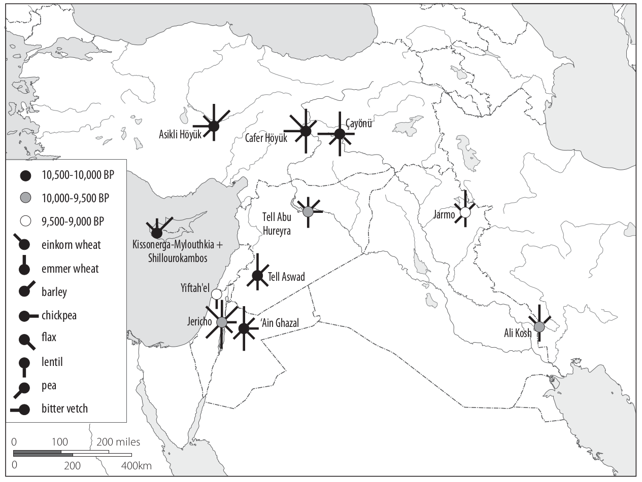
The archaeological findings can be summarized as follows:

First appearance in Near East: 17,000 - 8,000 BC. Brittle, two rowed-forms, similar to current wild barley. Likely collections of wild barley.
Oldest finding: Ohalo II, Sea of Galilee
First non-brittle barley: 7,500 BC in Tell Abu Hureyra (Syria)
Then in Tell Aswad (6,900-6,600 BC) (Syria) and Jarmo, Iraq (6,400 BC)

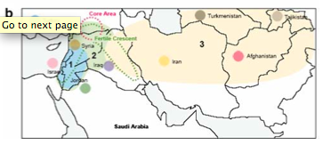
A map of the archeological sites with evidence of barley and other crops is shown in Figure 18

Figure 18: Archaeological sites in which barley was found. Source: Zohary D (2012)

In contrast, genetic studies suggest many more areas of barley domestication.

The strongest evidence was provided for the Near East Badr et al. (2000), but other locations were the Himalayas, North Africa / Spain, Ethiopia, because all of these regions are centers of cultivated barley diversity and areas in which wild barley occurs. However, the studies that postulate barley domestication outside the Fertile Crescent suffer from problems with the numbers and types of genetic markers as well as with the sampling. The best early study on barley domestication was by Badr et al. (2000).

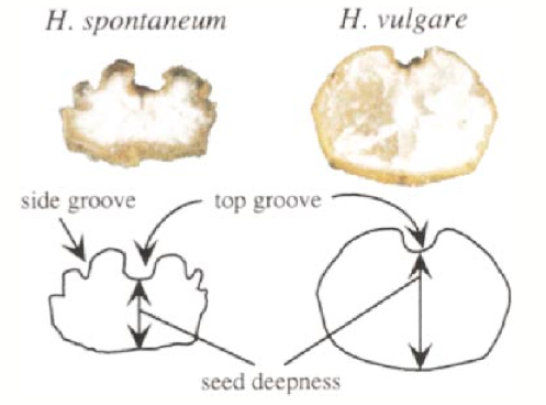
They used morphologial measurements of seeds to differentiate between wild and domesticated barley varieties and subsequently genotyped the ‘pure’, non-admixed lines with AFLP markers, and also analysed them morphologically.

Figure 19: Cross sections through barley grains to identify admixed (wild *H. spontaneum* vs. cultivated *H. vulgare*) genotypes. Source: Badr et al. (2000)

The results of the subsequent genotyping with AFLP markers suggest a single domestication event in the Near East, which was supported by later analyses (Figure 20).

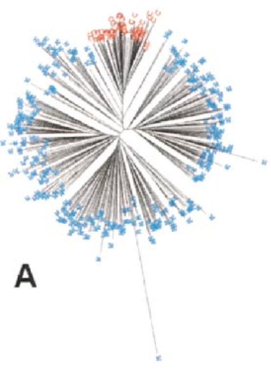
Figure 20: AFLP marker analysis of wild and domesticated barleys suggesting a single domestication event in the Near East. Source: Badr et al. (2000)

However, Badr et al. (2000) found some evidence of a secondary domestication event or a gene flow event in the Himalayan region by an AFLP marker analysis and the sequencing of a candidate gene.

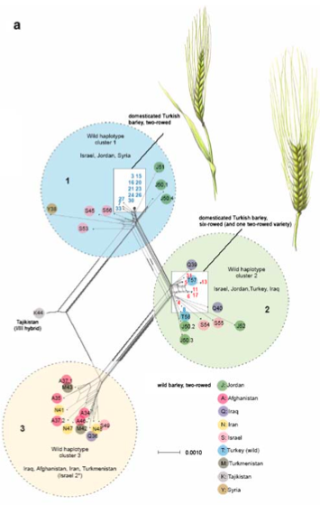
Figure 21: Phylogenetic network of wild barley from different regions in the distribution range indicating phylogenetic conflicts and evidence of gene flow. Source: Kilian et al. (2006)

Figure 22 shows the geographic distribution of the samples analysed in Figure 21.

Figure 22: Geographic origin of the accessions shown in Figure 21. Source: Kilian et al. (2006)

Another question investigated was the origin of two and six-rowed barley. The difference is due to a mutation in a single gene (Vrs1), which suggests that it originated once during barley evolution. This hypothesis is largely confirmed in a phylogenetic analyses, but there are also conflicting phylogenetic signals, possibly because of gene flow between the two types of cultivars.

The detailed analysis of a single gene showed evidence for gene flow. The Hooded (K) barley mutant phenotype is characterized by the formation of an ectopic flower at the lemma-awn interface, and it has been shown to be caused by a mutation in the Bkn-3 gene, which belongs to the Knotted-1-like-homeobox (Knox) gene class.

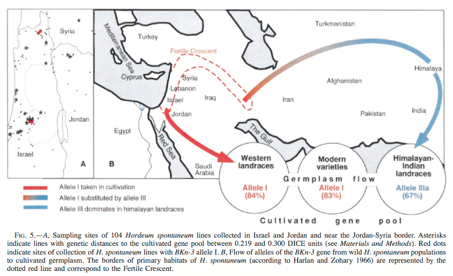
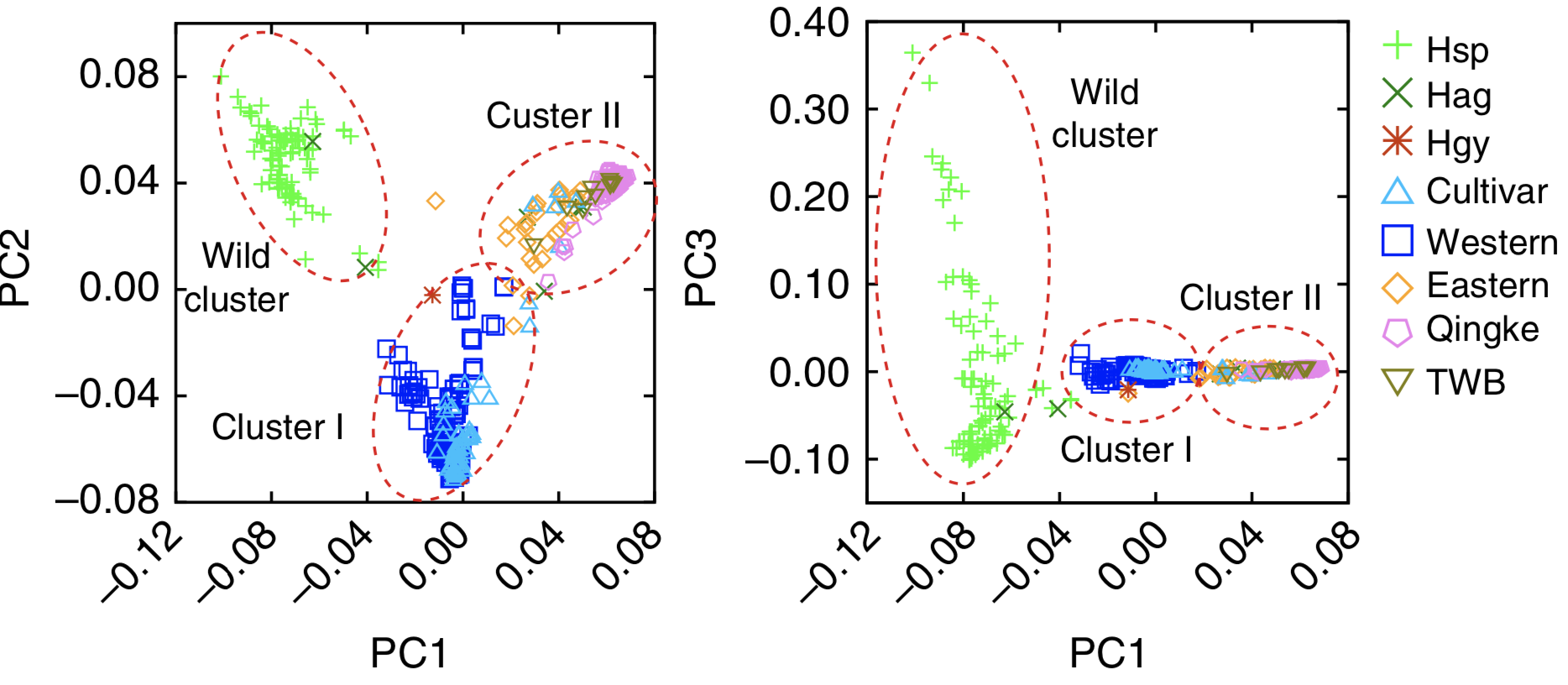
Figure 23: A hypothesis of gene flow of different alleles of the *Bkn-3* gene into barley landraces. Source: Badr et al. (2000)

Meanwhile, the hypothesis of a second domestication of barley in the Himalayas has been refuted (Zeng et al., 2018). Tibetan barley shows a low genetic diversity and is more closely related to barley landraces from the Fertile Crescent than to wild barley (Figure 24). The higher genetic diversity in Tibetan weedy barley is likely the result of feralisation (outcrossing) of cultivated barley with local wild barley genotypes.

Figure 24: PCA showing the close relationship between barley landraces from the Fertile Crescent and from Tibet. Source: Zeng et al. (2018).

Gene flow in bread wheat

Bread wheat has quite a heavy pollen, which is a consequence of its high ploidy level. It also has a limited longevity, which is about 30 min after dehiscence at field conditions with 20-30°C temperature. Under cooler, more optimal conditions, the longevity of functional pollen is not longer than 3 hours.

Bread wheat is a hexaploid crop ($2n=6x=42$, AABBDD) and is primarily self-fertilizing (autogamous). In the field, outcrossing rates are very small at 0.1%, under humid conditions, they can exceed 10% for certain genotypes. The same is true for most land races and wild Triticum and Aegilops relatives, except for Ae. speltoides Tauschii, which is typically allogamous.

Bread wheat is highly adapted to, and dependent from human cultivation. There is no evidence that with the correct cultivation method, feral wheat plants are maintained in the field. The weediness potential is limited as hexaploid plants are weak competitors and because they lack weediness traits.

Weediness traits include:

Prolonged seed dormancy
Extended persistence in the soil
Germination under a broad range of environmental conditions,
Rapid vegetative growth
A short life cycle
Very high seed output,
A high rate of seed dispersal
Long-distance seed dispersal

However, many wild relatives are colonizers and can invade new areas quickly.

Several Aegilops species have become troublesome weeds in North America, but not in Europe.

Gene pools of bread wheat

Due to the complex speciation history, bread wheat has a large gene pool 1 and 2. The species of gene pool 1 are shown in Table Table 2 and the species of gene pool 2 in Table Table 3.

Table 2: Summary of species in gene pool 1 of bread wheat, Triticum aestivum. Source: Andersson and de Vicente (2010)

Latin name	Common name	Genome
Triticum aestivum	bread wheat	AABBDD
T. zukovski	Zanduri wheat	AAAAGG
T. turgidum ssp. durum	durum wheat	AABB
T. turgidum ssp. dicoccum	emmer wheat	AABB
T. turgidum ssp. dicoccoides	wild emmer	AABB
T. timopheevii ssp. timopheevii	part of Zanduri wheat	AAGG
T. timopheevii ssp. armeniacum	wild emmer
T. monococcum ssp. monococcum	cultivated einkorn wheat	AA
T. moncoccum ssp. aegilopoides	wild einkorn	AA
T. uartu		AA

GP1 has the following characteristics:

Hexaploid wheats can be crossed easily and result in fertile and viable progeny.
Diploid and tetraploid forms are interfertile with bread wheat, but to a lesser extent and the fertility of the F1 hybrids is often reduced.
Offspring with diploid forms is less fertile than with tetraploid forms. Fertility can be restored by backcrosses or chromosome doubling.

GP2 consists of geographically widely distributed species of the genus Aegilops (Table Table 3) and are very numerous.

Table 3: Summary of species in gene pool 2 of bread wheat, Triticum aestivum. Source: Andersson and de Vicente (2010)

Latin name	Genome	Species
Aegilops ssp.	U genome	8
	M and N genomes	2
	C genome	2
	D genome	5
	S genome	5
	T genome	1
Total:		23

The direction of the cross is also important. Crosses with the diploid D-genome donor Aegilops tauschii also require manipulation and artificial hybridization. Synthetic hexaploids have been produced which are then crossed to hexaploid cultivars.

Triticale is a human-made cereal resulting from a cross of bread or durum wheat with rye Secale cereale and occurs as tetraploid, hexaploid and octoploid forms. There is a certain extent of cross compatibility with wheat and rye; some spontaneous hybridization with wheat occurs in the field. With artificial techniques, triticale can be used as a bridge for introgression between rye and wheat.

To summarize, wheat can be crossed with most of wild and cultivated GP1 relatives. But frequently artificial techniques are required. Spontaneous hybridization and gene transfer in the field occurs for some combinations, but is unlikely. Among GP2 species, some spontaneous hybridizations occurred with Aegilops species.. %However, the process can be quite complex. There is no evidence for natural hybridizations with GP3 (more distant grass species), but some can be generated artificially, such as with rye to produce triticale.

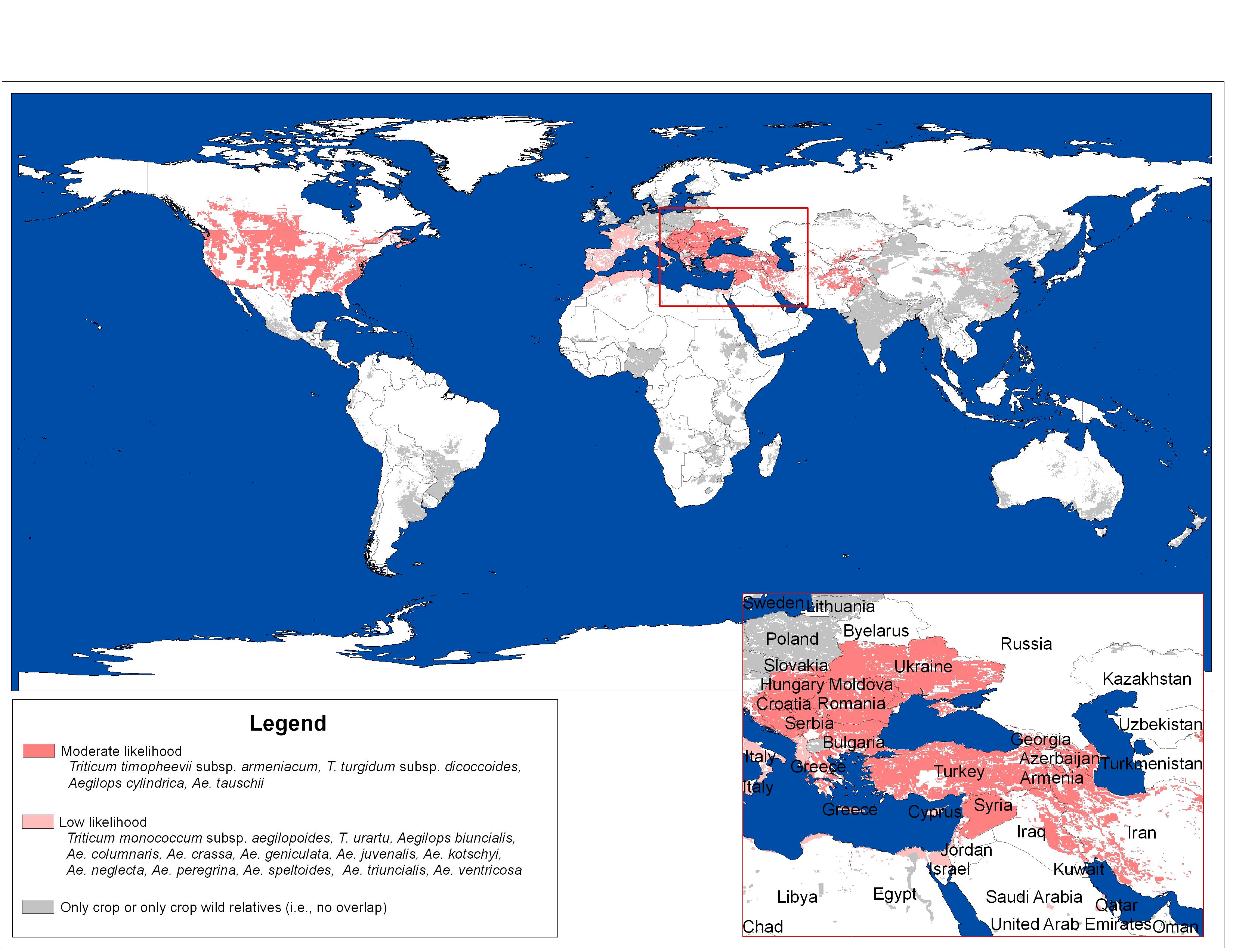
Figure 25 shows a map with the potential chance (or risk) of gene flow between bread wheat and species from the extended gene pool.

Figure 25: Map of the distribution of close relatives of wheat. These species can be potentially used as genetic resources by introgresson. Source: Andersson and de Vicente (2010)

The following two tables show the full list of species from GP1 and GP2 of wheat.

Figure 26: Species of GP1. Source: Andersson and de Vicente (2010)

Outcrossing rates and distances

An assessment of gene flow and the potential of hybridization is very important in the production of seeds and an evaluation of the risk for outcrossing of GMO varieties.

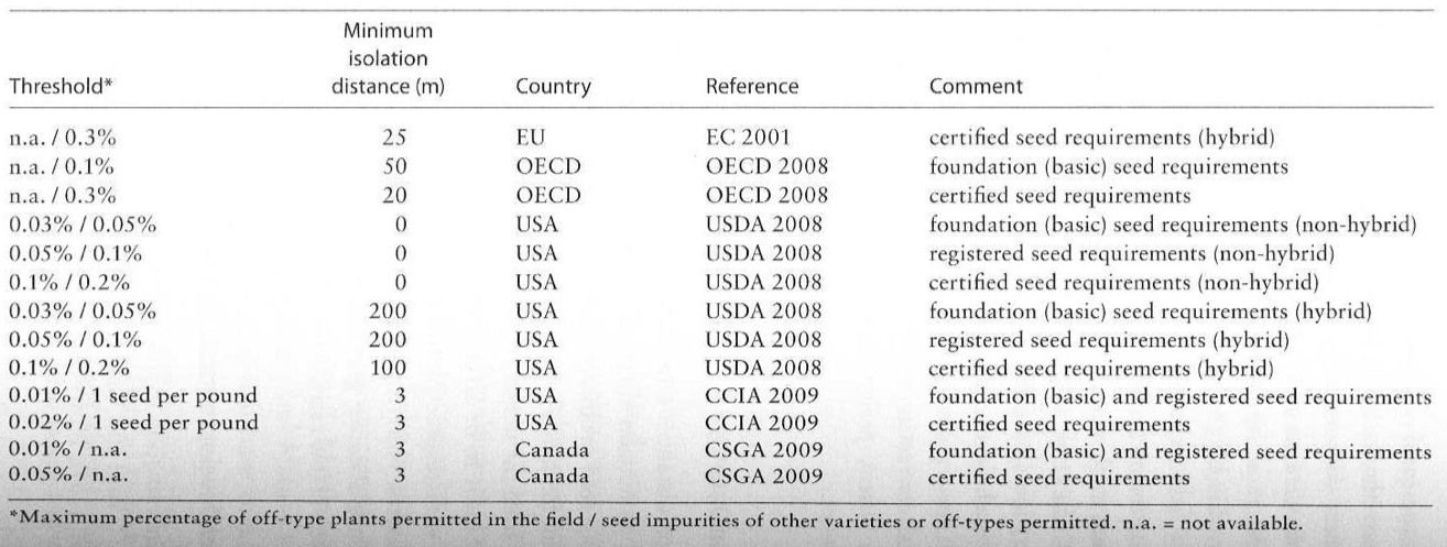
In field experiments, pollen flow between plants more than 30 m apart is usually not observed. In some studies, cross fertilization was detected at distances exceeding 40-60 m, in some very rare cases even $>$ 2.75 km from the pollen source at very low rates ($<0.01$%). For seed production, official distances vary from 3 to 50 for normally fertile varieties and from 25 to 200 m for hybrid seed production. Separation distances of 30 m are likely to be effective both for maintaining seed-purity standards and with respect to the maximum allowances (0.9%) from GM trait admixtures (Table Table 4). But gene flow is strongly influenced by environmental conditions.

Table 4: Isolation distances. Source: Andersson and de Vicente (2010)

Most spontaneous outcrossing is expected with tetraploid Aegilops species.

For this reason, the risk of introgression is highest in regions where bread wheat and Aegilops co-occur (Figure 25).

Key concepts

$\square$ Gene flow	$\square$ Reticulate evolution	$\square$ Polyploidization
$\square$ Phylogenetic network	$\square$ Incomplete lineage sorting	$\square$ Shared ancestral variation

Summary

Gene flow and reticulate evolution cause a deviation from a simple, bifurcating model of genetic divergence within and between species.
The extent of gene flow depends on intrinsic and extrinsic factors.
Polyploidization and hybridization are important events in the evolution of crop plants or their ancestors.
There are direct and indirect methods to measure gene flow. Direct methods allow to estimate current rates of gene flow, whereas indirect methods analyse recent and historical rates of gene flow.
By which criterion are the A, B and D genomes of bread wheat defined?

Study questions

What is the difference between gene flow and hybridization?
What are the differences between auto- and allopolyploidy?
What is a phylogenetic incongruence?
Why are strictly bifurcating trees misleading in the presence of gene flow?

Problems

Read the abstract and check out 5 of the paper by Glémin et al. (2019). What are the key messages of their study? What do their results implicate for the use of crop wild relatives of wheat? Can you develop a research strategy that uses these resources and will contribute to the diversification of wheat breeding for future climatic conditions and agronomic systems? Link to article: https://advances.sciencemag.org/content/5/5/eaav9188
Read the abstract and check out 4 of the paper by Stetter et al. (2017) on the domestication of South American grain amaranth. Describe the key result that is evident from the figure How does the phylogenetic figure support or not support the claim of incomplete domestication? Can you think of alternative explanations for the observed patterns.

Exercises

Discussion questions

Discuss the questions in small groups of 2–3 students:

What is the difference between gene flow and hybridization?
What are the differences between auto- and allopolyploidy?
What is a phylogenetic incongruence?
Why are strictly bifurcating trees misleading in the presence of gene flow?

Interpretation of a diversity study

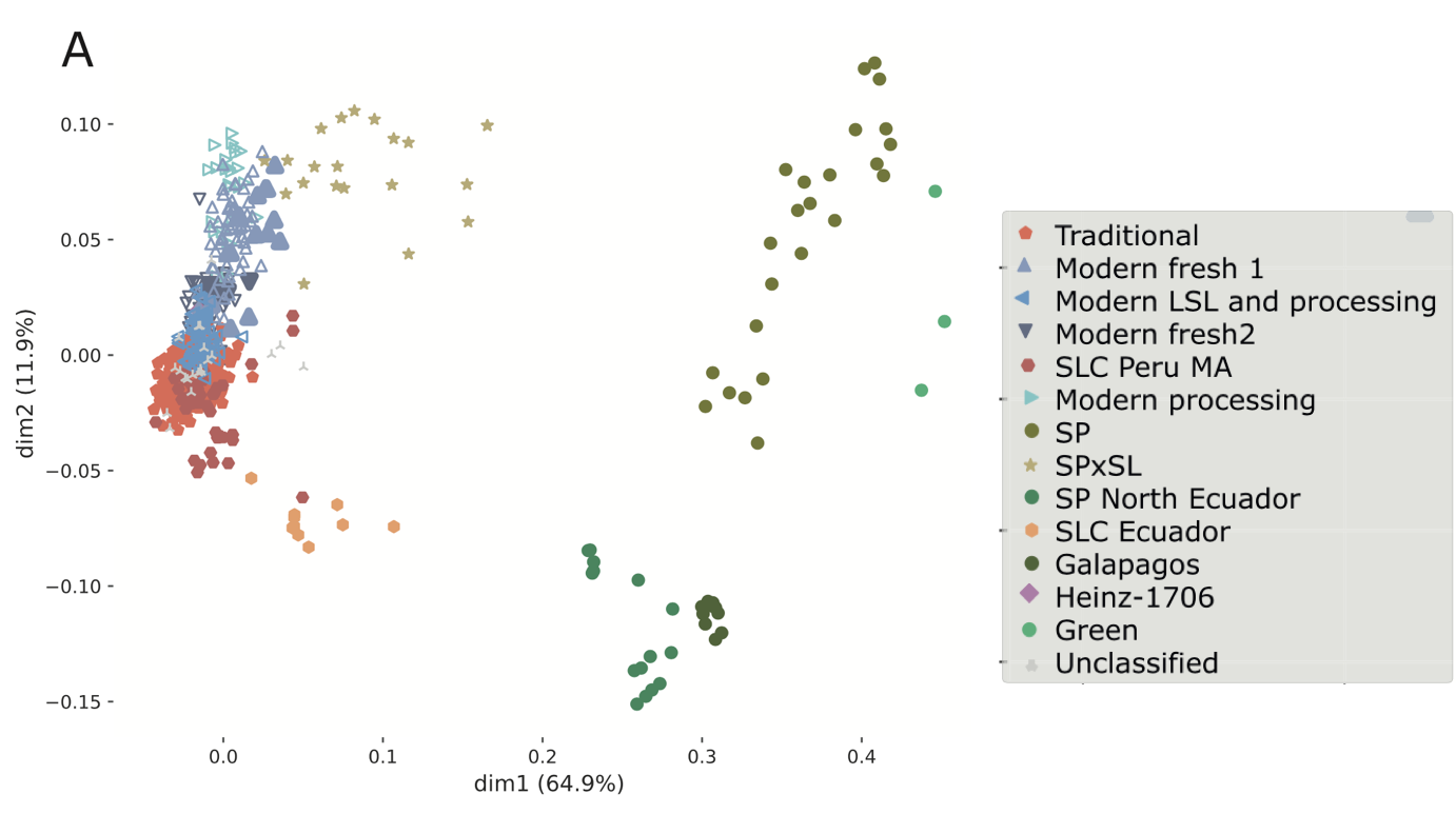
Blanca et al. (2022) genotyped a set of 1,254 tomato accessions including European traditional and modern varieties, early domesticated varieties and wild relatives with the following results:

There was a continuous genetic gradient between traditional and modern varieties
European traditional varieties had a very low genetic diversity
European traditional varieties clustered into several genetic groups with Spanish and Italian varieties showing a higher genetic diversity than remaining varieties: they have a complex migration and hybridization pattern.
Loci with association morphological traits showed a significantly higher diversity: Evidence for balancing selection.

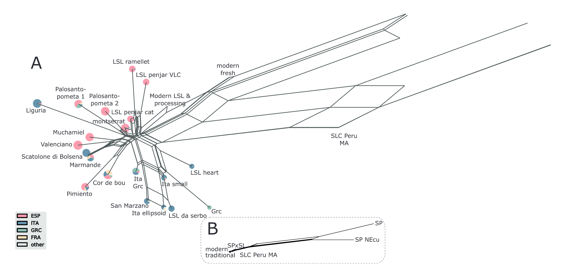
Some key results are presented in the two figures.

Figure 27: Principal coordinate analysis (PCoA) including cultivated tomato (*Solanum lycopersicum* var. *lycopersicum*; SLL): traditional European tomato, modern cultivars with different culinary use [fresh, processing, and long shelf-life (LSL)]; *Solanum lycopersicum* var. *cerasiforme* (SLC) from different origins [Peru, Mesoamerica (MA), Ecuador]; and several American wild relatives: *Solanum pimpinellifolium* (SP), *Solanum cheesmaniae*, *Solanum galapagense* (Galápagos), *Solanum peruvianum*, *Solanum chmielewskii*, *Solanum habrochaites* (Green), and SP×SL hybrids. The modern cultivar Heinz 1706 was included as reference. Empty symbols indicate accessions initially reported as traditional but reclassified as modern. (A) First and second principal components (dim1 and dim2) from the PCoA using all accessions analyzed in this study.

Figure 28: Evolutionary relationships between traditional European tomato, modern tomato, and Peru and Mesoamerica *Solanum lycopersicum* var. *cerasiforme* (SLC), *Solanum pimpinellifolium* (SP), and SP×SL hybrids. Split network based on the Dest distances between genetic groups. The country of origin of accessions within each genetic group is represented by a pie chart (colors are defined in the key shown in the bottom left). (A) Zoom only on European modern and traditional tomatoes. (B) Zoom on American ancestral and wild tomatoes. Each edge of the network represents a split of the accessions based on one or more characteristics. If there was no conflict, each split is represented by a single edge, whereas in the case of contradictory patterns the partition is represented by a set of parallel edges. The edge lengths represent the weight of each split, which is equivalent to the distance between groups. ESP, Spain; GRC, Greece; FRA, France; ITA, Italy; LSL, long shelf-life; MA, Mesoamerica; NEcu, North Ecuador; VLC, Valencia (Spain).

Please answer the following questions:

Summarize the results of Figure 27 in a few sentences.
Which conclusions does the figure allow with respect to the relationship of groups of tomato cultivars and the genetic diversity of the groups?
Which information can not be obtained from Figure 27 about the history and diversity of tomatoes?
Summarize the results of Figure 28 in a few sentences.
Which information can be obtained on the relationship and gene flow among tomato varieties?
Which information can not be obtained from the figure?

References

Acquaah G. 2009. Principles of plant genetics and breeding. John Wiley & Sons.

Andersson M, de Vicente M. 2010. Gene Flow between Crops and Their Wild Relatives. Johns Hopkins.

Arbogast BS, Edwards SV, Wakeley J, Beerli P, Slowinski JB. 2002. ESTIMATING DIVERGENCE tIMES fROM MOLECULAR DATA oN pHYLOGENETIc AND POPULATION gENETIC TIMESCALES. Annu Rev Ecol Syst 33:707–740. doi:10.1146/ecolsys.2002.33.issue-1

Badr A, Müller K, Schäfer-Pregl R, Rabey HE, Effgen S, Ibrahim HH, Pozzi C, Rohde W, Salamini F. 2000. On the origin and domestication history of Barley (Hordeum vulgare). Mol Biol Evol 17:499–510.

Blanca J, Pons C, Montero-Pau J, Sanchez-Matarredona D, Ziarsolo P, Fontanet L, Fisher J, Plazas M, Casals J, Rambla JL, Riccini A, Pombarella S, Ruggiero A, Sulli M, Grillo S, Kanellis A, Giuliano G, Finkers R, Cammareri M, Grandillo S, Mazzucato A, Causse M, Díez MJ, Prohens J, Zamir D, Cañizares J, Monforte AJ, Granell A. 2022. European traditional tomatoes galore: A result of farmers’ selection of a few diversity-rich loci. Journal of Experimental Botany erac072. doi:10.1093/jxb/erac072

Chen ZJ. 2007. Genetic and epigenetic mechanisms for gene expression and phenotypic variation in plant polyploids. Annu Rev Plant Biol 58:377–406. doi:10.1146/annurev.arplant.58.032806.103835

Cranston KA, Hurwitz B, Ware D, Stein L, Wing RA. 2009. Species Trees from Highly Incongruent Gene Trees in Rice. Systematic Biology 58:489–500. doi:10.1093/sysbio/syp054

Glaszmann JC, Kilian B, Upadhyaya HD, Varshney RK. 2010. Accessing genetic diversity for crop improvement. Current opinion in plant biology 13:167–73. doi:10.1016/j.pbi.2010.01.004

Glémin S, Scornavacca C, Dainat J, Burgarella C, Viader V, Ardisson M, Sarah G, Santoni S, David J, Ranwez V. 2019. Pervasive hybridizations in the history of wheat relatives. Science Advances 5:eaav9188. doi:10.1126/sciadv.aav9188

Hey J, Machado CA. 2003. The study of structured populations — new hope for a difficult and divided science. Nature Reviews Genetics 4:535–543. doi:10.1038/nrg1112

Kilian B, Özkan H, Kohl J, Haeseler A, Barale F, Deusch O, Brandolini A, Yucel C, Martin W, Salamini F. 2006. Haplotype structure at seven barley genes: Relevance to gene pool bottlenecks, phylogeny of ear type and site of barley domestication. Mol Genet Genomics 276:230–241. doi:10.1007/s00438-006-0136-6

Loisel DA, Rockman MV, Wray GA, Altmann J, Alberts SC. 2006. Ancient polymorphism and functional variation in the primate MHC-DQA1 5’ cis-regulatory region. Proceedings of the National Academy of Sciences 103:16331–16336.

Lowe A, Harris P, P A. 2004. Ecological genetics: Design, analysis and application. Oxford: Blackwell.

Posada D, Crandall K. 2001. Intraspecific gene genealogies: Trees grafting into networks. Trends in ecology & evolution 16:37–45.

Salamini F, Ozkan H, Brandolini A, Schäfer-Pregl R, Martin W. 2002. Genetics and geography of wild cereal domestication in the near east. Nature Reviews Genetics 3:429–41. doi:10.1038/nrg817

Stetter MG, Müller T, Schmid KJ. 2017. Genomic and phenotypic evidence for an incomplete domestication of South American grain amaranth (Amaranthus caudatus). Molecular Ecology 26:871–886. doi:10.1111/mec.13974

Zeng X, Guo Y, Xu Q, Mascher M, Guo G, Li S, Mao L, Liu Q, Xia Z, Zhou J, Yuan H, Tai S, Wang Y, Wei Z, Song L, Zha S, Li S, Tang Y, Bai L, Zhuang Z, He W, Zhao S, Fang X, Gao Q, Yin Y, Wang J, Yang H, Zhang J, Henry RJ, Stein N, Tashi N. 2018. Origin and evolution of qingke barley in Tibet. Nature Communications 9:1–11. doi:10.1038/s41467-018-07920-5

Zohary D WE Hopf M. 2012. Domestication of Plants in the old world, 4th ed. Oxford University Press.

\(\square\) Gene flow	\(\square\) Reticulate evolution	\(\square\) Polyploidization
\(\square\) Phylogenetic network	\(\square\) Incomplete lineage sorting	\(\square\) Shared ancestral variation

Gene flow