Coalescent theory

Motivation: Looking back in time

The analysis of genetic variation with simple descriptive statistics such as Nei's gene diversity in genetic resources and breeding material may be sufficient for many practical purposes related to the characterization of PGR or for plant breeding. Since current patterns of genetic variation are the result of past historical processes, the analysis of the evolutionary history of a population may provide additional insights.

Therefore the question arises: How are current patterns of genetic variation linked to evolutionary processes in the past? This can be shown with the example in Figure 1 which shows the connection of individidual buttervlies to phylogenetic processes.

Figure 1: Individuals living in the present are connected by evolutionary processes. Source: Maddison and Maddison (1992)

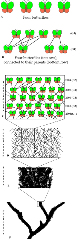
Four butterflies (and the genetic diversity they represent) sampled from a population are connected on a short evolutionary time scale (e.g., measured in generations) by familial relationships (e.g., via their parents), but in the long term are also connected and influenced by other evolutionary process that influence populations and species.

These concepts are relevant if the goal is to identify useful genetic variation in plant genetic resources or to predict the change in genetic variation under different types of germ plasm management or in plant breeding programs.

The models used in classical theoretical population genetics allow to model future changes in allele frequencies. For this reason, they are prospective.

In contrast, the analysis of real populations is based on samples taken taken from the population. The patterns of polymorphism observed in the sample are then used to identify evolutionary processes that acted in the past. Therefore, the perspective is retrospective by looking back in time.

Unfortunately, processes that acted in the past are unknown and can not be directly observed. For this reason, population genetic analyses attempt to infer past evolutionary processes. A typical example is the question whether the population size of a species was reduced for a certain number of generations or whether a species has expanded its range in recent times. Coalescent theory was developed to achieve this goal. In the following, the key principles and mathematical properties of the coalescent will be derived.

Learning goals

1. Understand the key principle underlying coalescent theory in the context of gene genealogies
2. Know the different roles of the genealogical and the mutational process in creating genetic diversity that are observed in population samples of genetic diversity
3. Understand the principles of inferring demographic parameters of populations using coalescent theory and simulations
4. Being able to apply coalescent theory in describing the genetic history of plant genetic resources

How to model data on genetic diversity

We start with a simple example. Assume a sample of four haploid chromosomes that have been sequenced at a locus, which identified three SNP polymorphisms. Further assume that no recombination occurs. Figure 2 shows on the right the three SNPs and the allel configuration (haplotypes) in four sequenced chromosomes. The left tree shows a possible gene genealogy of the locus and the branches on the tree on which the mutations occurred and were subsequently inherited to the descending lines.

Figure 2: Linking observed sequence variation with gene genealogies and mutations. A locus has been sequenced in a sample of four chromosomes, in which 3 SNPs are segregating.

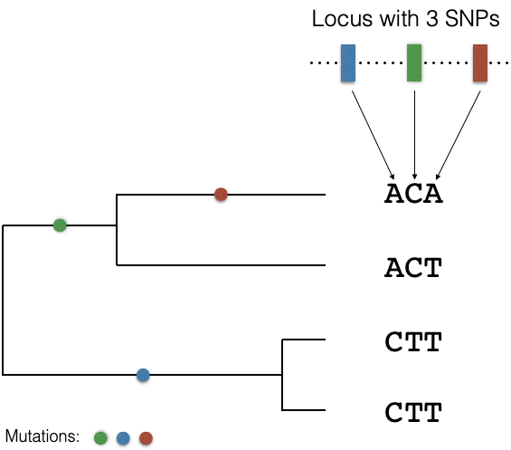
The ancestry (past evolutionary history) of the observed diversity in Figure 2 can be analysed by two approaches:

First, one could follow a phylogenetic approach: Use the data to try to reconstruct the real ancestral that expresses the evolutionary relationship among the four haplotypes. This will provide information on the particular evolutionary history of the locus.

Second, apply coalescence theory: Give only constraints for the ancestral tree and estimate the likelihood of the tree given the constraints (or model parameters). For example, one may ask how likely the observed number of three SNPs in a gene of 1,000 bp length is under a neutral model (i.e., no selection) of a constant population size and a genome-wide level of the population mutation parameter $\theta =4N_e\mu$. By following this approach, our goal is not to reconstruct the history of the given sample, but rather ask which process(es) produce the observed data with the highest likelihood. Then, we may learn something about evolutionary processes (selection, drift, etc.) that acted in the past to shape the genetic diversity we observe in the present.

The Wright-Fisher model

To develop the key principles of coalescent theory we introduce the Wright-Fisher model, which is an important model for modeling evolutionary process in populations of finite size and discrete populations.¹

¹ The model is named after the two evolutionary biologists Sewall Wright and Ronald Fisher who developed the foundations for theoretical population genetics.

The model assumes a finite number of individuals $N$ with $2N$ chromosomes in diploid individual. These individuals produce an infinite number of gametes, from which $2N$ gametes are randomly drawn to produce $N$ offspring in the next generation (Figure 3). Note, that in this model the population size remains constant over generations.

Figure 3: Scheme of a Fisher-Wright model over 2 generations.

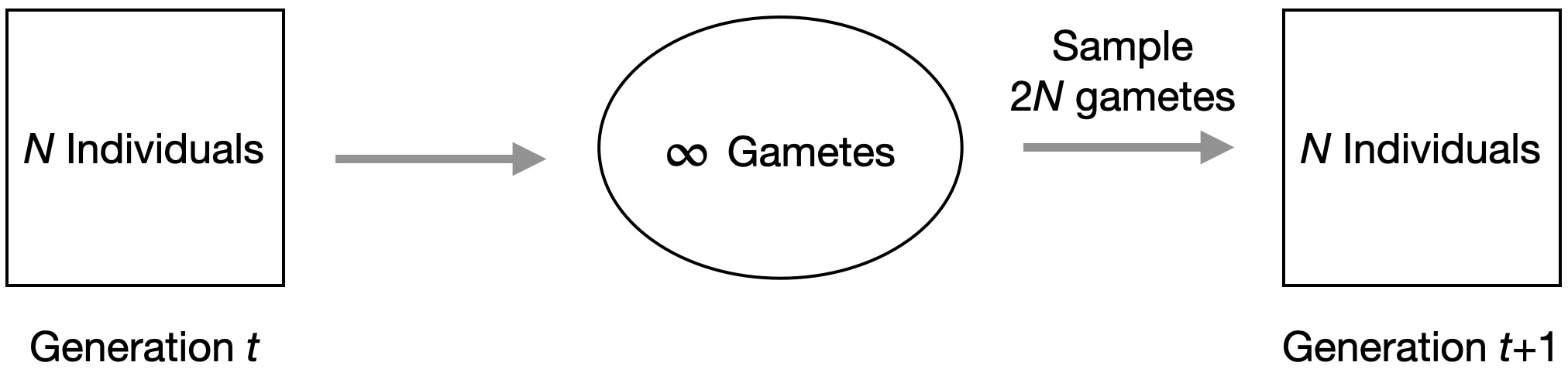
By assuming an independent number of gametes, the probability that two randomly drawn chromosome derive from the same parental chromosomes is $1/2N$. In other words, $1/2N$ is the probability that to alleles are identical by descent (IBD)² In addition, the probability that a randomly drawn gamete has allele $A_1$ at locus $A$ corresponds to the frequency of the allele in the population.

² The concept of IBD is fundamental in population genetics, and you should understand its meaning and consequences. For example check out the corresponding chapter in the module “Population and Quantitative Genetics” on inbreeding.

Let us summarize the Wright Fisher-Model:

• It is a population model for $N$ individuals with $2N$ alleles. $N$ remains constant.
• Alleles in the next generation are randomly sampled from the previous generation.
• Therefore, probability that two alleles share the same parental allele: $\frac{1}{2N}$

Our goal is investigate the history of a sample of $n$ alleles backwards in time. We assume the sample is much smaller than the population size $N$, therefore $n\ll N$.

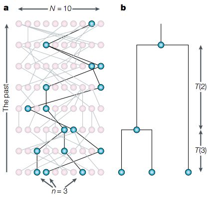
The model can then be used to model the properties of a sample, as shown in Figure 4.

Figure 4: Properties of a sample created under the Wright-Fisher model.

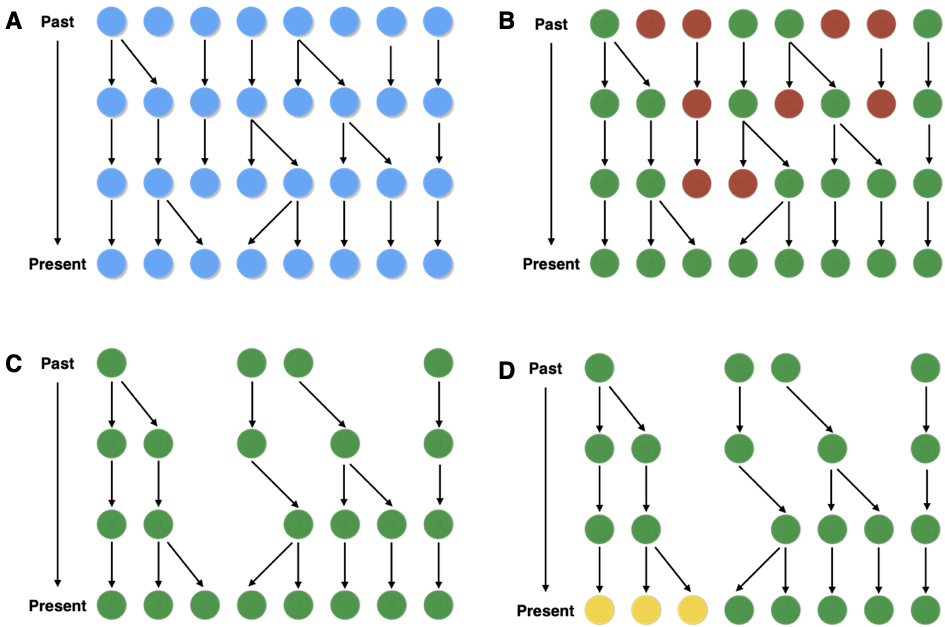
Figure 4 shows a sample of three haploid chromosomes ($n=3$) from a population of $2N=8$ chromosomes (under the assumption of a diploid species) separated by discrete generations. The individuals are related by a genealogical relationship, which allows that some chromosomes are descendants of the same parental chromosome. Using this genealogical structure, time is measured backwards (in generations) and the observed ancestral tree resembles a random tree generated under the Fisher-Wright model.

The key principle of coalescent theory

The analysis of genetic variation in a historical context can be achieved by combining the genealogical process with the process of mutation:

Genealogical process:

All chromosomes of a population sample have an evolutionary relationship that can be represented as a phylogeny or a gene genealogy. The true genealogy is unknown.

Process of mutation:

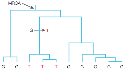
A genetic polymorphism in a sample of alleles from a population results from a mutation that occurred on a certain branch on a genealogical tree (Figure 5). All descendants of this lineage carry this mutation.

Figure 5: Origin of genetic variation.The mutation on a particular branch of the phylogenetic tree is shown as G $\to$ T. The tree connects sampled individuals at the basis, which represents the most recent common ancestor. Source: Rosenberg and Nordborg (2002)

Coalescence theory attempts to investigate how the current composition of alleles in a population is the result of these to process processes that acted in the past of a population, from which a sample was taken. It is the most important tool in the reconstruction of the genetic history of a population. It is achieved by reducing the evolution of a population to its genealogy. Alleles that trace back to a common ancestor a few generations ago are more closely related to each other than other alleles.

Figure 6: The basic principle of the coalescent. (A) A genealogy of ten haploid individuals is shown (diploid populations of $N$ diploid individuals are usually studied as a population of $2N$ haploid individuals. Three individuals are sampled in this population. (B) The subtree of the sampled individuals with their coalescent times is shown. Source: Rosenberg and Nordborg (2002)

Each time when two alleles trace back to a common ancestor in a gene genealogy, one speaks of a coalescent event. At one point in the past all alleles in a sample coalesced to a single common ancestor, which is called most common recent ancestor (MRCA). The sum of all coalescent events is called the coalescent. The key advantage of coalescence theory is shown in Figure 6: One does not need to investigate the whole population to make inferences, but can rely on a much smaller sample from the population.

Coalescence theory was introduced into population genetics by the English mathematician John Kingman in 1982 (Kingman, 1982). The abstract and theoretical nature of coalescent theory does not diminish its great importance for molecular population genetics and in practical applications.

The coalescent and gene genealogies

The coalescent of a sample is called its genealogy because it shows the genealogical relationship of the alleles in the sample. Of course, the true genealogy and its coalescence events are not known: It can not be determined which alleles had common ancestors, and the time points of coalescent events are not known.

All of these parameters have to be estimated from the observed data. Coalescent theory provides a framework to estimate these parameters.

Probability of coalescent events

Coalescent theory attempts to estimate probabilities and the time points of coalescent events in a genealogy. Assume a diploid population of size $N$ that evolves under a Wright-Fisher model It is further assumed that the sequences of a locus evolve neutrally (without selection); in this case one speaks of a neutral coalescent.

Figure 7 shows a neutral genealogy of a sample of five alleles that was taken from a Wright-Fisher population.

Figure 7: A typical gene genealogy of a sample of five alleles that evolve according to the neutral coalescent process.

We no calculate the probability that a coalescence event happens, i.e., that two alleles are identical by descent (IBD) because they have the same ancestor in the previous generation. This probability is $1/2N$ in diploid species and is calculated as follows:

1. Randomly sample a single gamete from the population, which corresponds to probability of 1.
2. Randomly sample a second gamete from the population. The probability that this gamete was derived from the same chromosome is $1/2N$.

Therefore, the total probability that two randomly drawn gametes coalesce in the previous generation (or are IBD) is $$\begin{array}{}\text{(1)}& P(\text{IBD})=1\times \frac{1}{2N}=\frac{1}{2N}\end{array}$$ The probability that no coalescence event happens in this generation is therefore $1-(1/2N)$.

In a sample of five alleles there are ten possibilities to form ($n(n-1)/2$) pairwise combinations.

For this reason, the probability of observing a coalescence event between any two alleles in a sample of $n$ alleles in the previous generation equals $$\begin{array}{}\text{(2)}& \frac{n(n-1)}{2}\frac{1}{2N}=\frac{n(n-1)}{4N}.\end{array}$$ In a population of 10,000 individuals and from which a sample size of five alleles this probability equals 1 in 4,000.

Time points of coalescence events

It is possible to calculate the probability that a coalescence event occured exactly $t$ generations ago. The probability that no coalescence event occurs in the first generation is $$\begin{array}{}\text{(3)}& 1-\frac{n(n-1)}{4N}\end{array}$$ The probability that a coalescent event occured $t$ generations ago is the probability that it did not occur in the first $t-1$ generations multiplied by the probability of this event in generation $t$.

If $p$ is the probabilty of a coalescence event in an arbitrary generation and $1-p$ the probability that it does not occur, the probability of a coalescence event in generation $t$ equals $$\begin{array}{}\text{(4)}& Pr(T_t)=(1-p{)}^{t-1}p\end{array}$$ with $T_t$ as the number of generations until the coalescence of $n$ to $n-1$ alleles.

Equation $\text{(4)}$ describes a geometric distribution in which the occurrence of a coalescence event is called a 'success'.

Geometric distributions have the following properties (Wikipedia):

• The mean of a geometric distribution is inverse to the probability of success, $1/p$
• The variance is $q/p^2$, where $q=1-p$ is the probability of no success

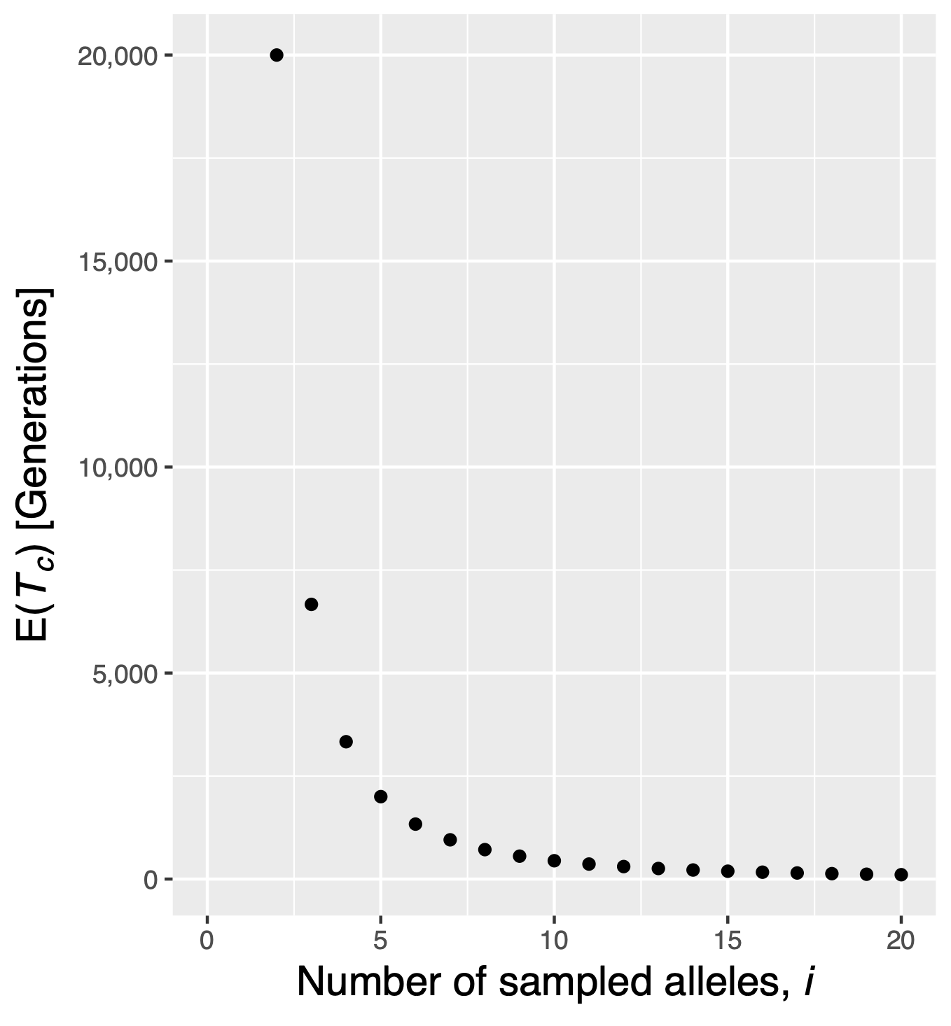
Remember that the probability of a coalescence event in a set of $n$ alleles in the previous generation is $$p=\frac{n(n-1)}{4N}.$$ From these properties it follows that the expected (i.e., mean) time to the first coalescence event is $$\begin{array}{}\text{(5)}& E(T_n)=\frac{1}{\left(\frac{n(n-1)}{4N}\right)}=\frac{4N}{n(n-1)}\end{array}$$ This can be further generalized, because $n$ can assume a value between 2 and infinity. The average time span of a coalescent event with $i$ alleles to one with $i-1$ alleles is then $$\begin{array}{}\text{(6)}& E(T_i)=\frac{4N}{i(i-1)}\end{array}$$ With Equation $\text{(6)}$ it is possible to answer the question of the average coalescence time of two randomly isolated alleles from a population. For $i=2$ the time is $2N$ generations. A comparison of different values of $i$ shows that $E(T_i)$ decays rapidly with increasing $i$ (Figure 8): With large sample sizes, the time to the first coalescence event is very short, i.e., only a few generations.

Figure 8: Expected time to first coalescent in number of generations for different number of sampled alleles as calculated with ?@eq-expectedtime. The population size is $N=10,000$.

Exercise

Calculate the expected time to the first coalescent event for the following sample and population sizes:

• $n=10$, $N=10,000$
• $n=100$, $N=10,000$
• $n=10$, $N=1,000,000$
• $n=100$, $N=1,000,000$

Which parameter (sample size $n$ or population size $N$) has a larger effect on the time to the first coalescent?

Coalescence times within a genealogy

Using Equation $\text{(6)}$ the distribution of coalescent times within a genealogy can be investigated. This is demonstrated by rewriting Equation $\text{(6)}$ to $$\begin{array}{}\text{(7)}& E(T_i)=\frac{4N}{i(i-1)}=\frac{2N}{\frac{i(i-1)}{2}}\end{array}$$ $E(T_i)$ is the average coalescent time of two randomly chosen alleles ($2N$) divided by the number of possible pairwise combinations of all alleles, $i$, among which coalescent events may occur.

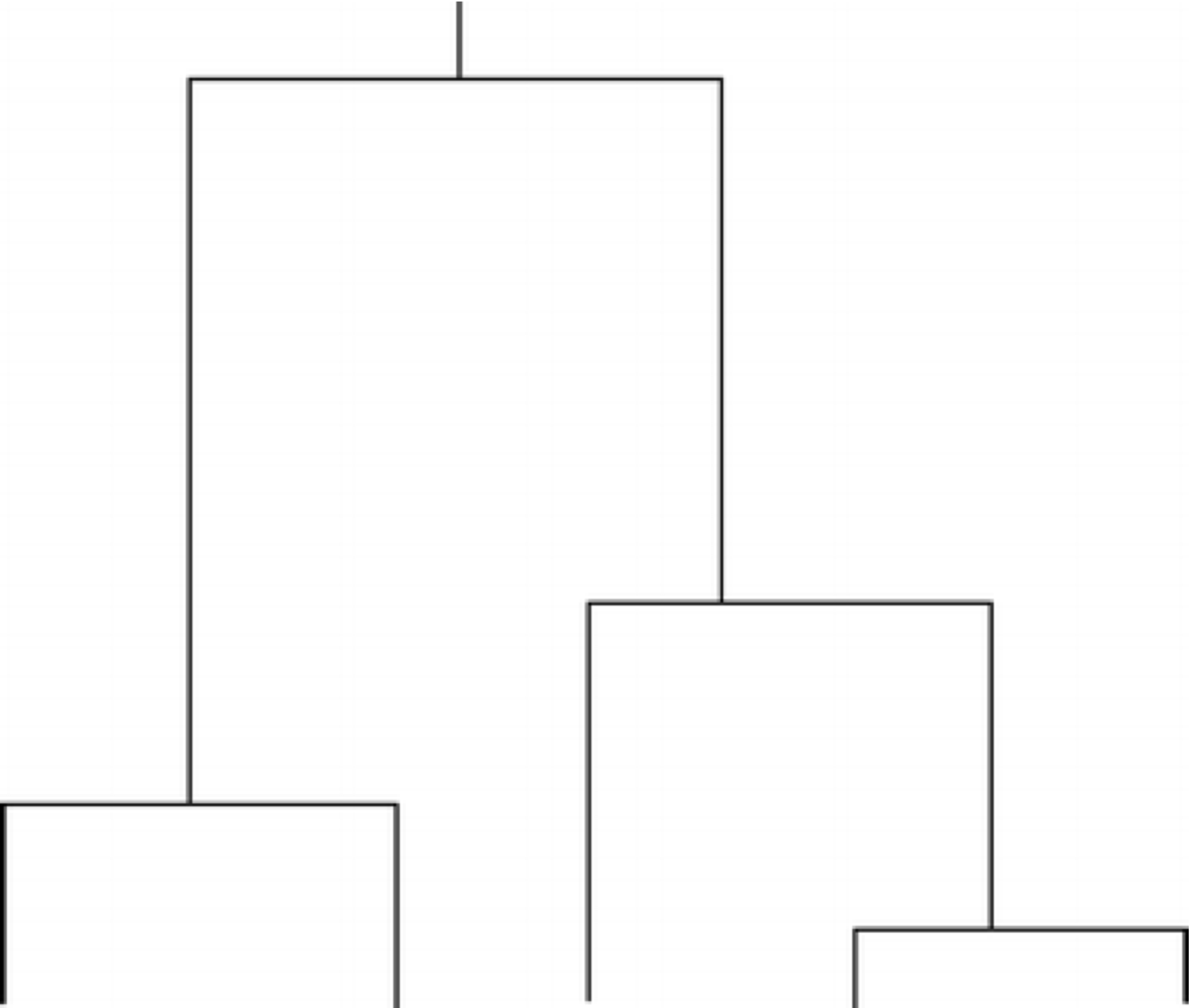
The number of such allele combinations is calculated as $$\begin{array}{}\text{(8)}& \left(\begin{array}{c}i\\ 2\end{array}\right)=\frac{i!}{(i-2)!2!}=\frac{i(i-1)}{2}\end{array}$$ Figure 9 shows the distribution of coalescence times in a genealogy.

Figure 9: Coalescence time in a gene genealogy. Source: Hartl and Clark (2007).

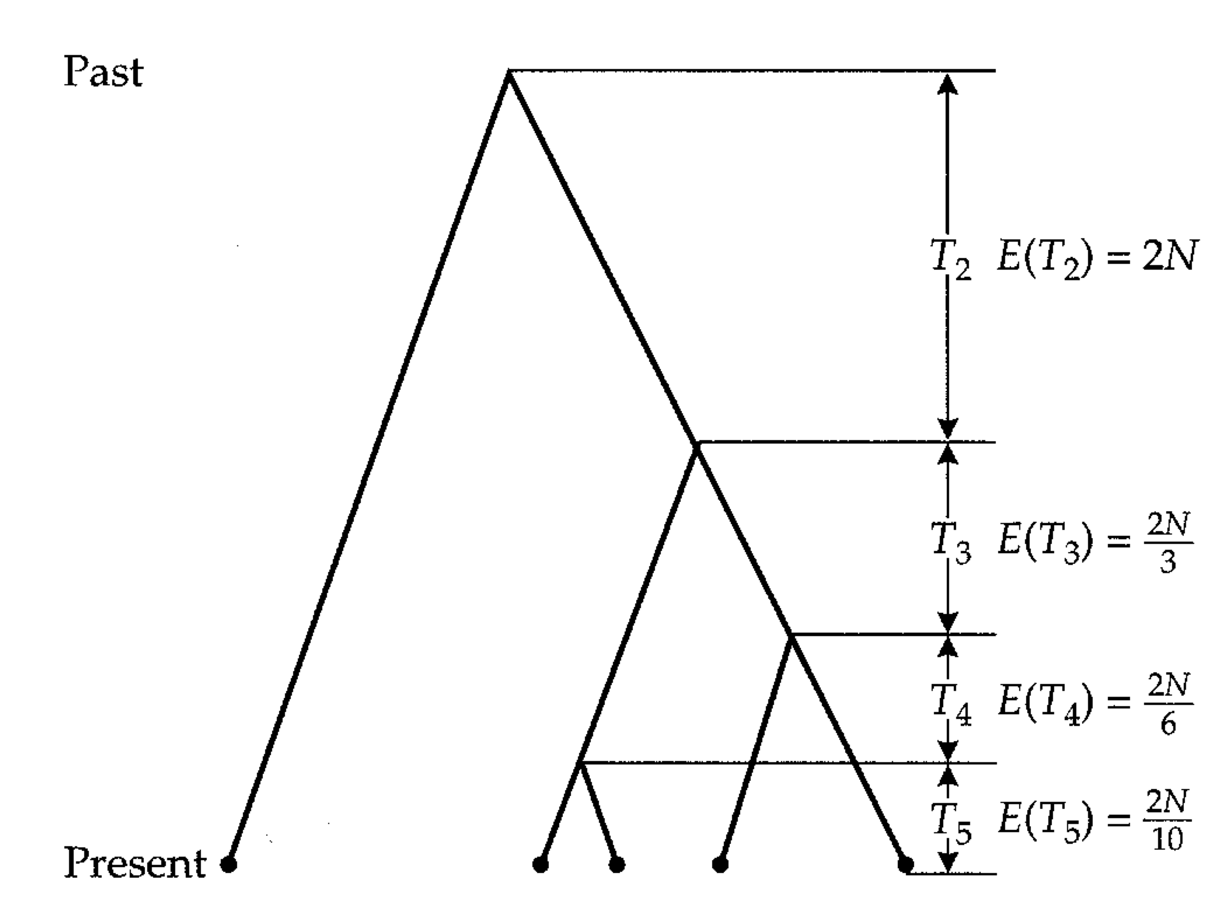
The intervals between coalescent events increase and the last coalescent event takes the longest time. For example, the times for a sample of five alleles ($n=4$) and a population size of 10,000 individuals ($N=10,000$) equals 2,000 generations for the first, 3,333 for the second and 6,666 for the third and 20,000 generations for the fourth coalescent event.

The total length of a genealogy

The total length of a genealogy, $T_c$, corresponds to the total time of all branches of a coalescent: $$\begin{array}{}\text{(9)}& T_c=\sum _{i=2}^{n}i{T}_i,\end{array}$$ By applying the rule that the sum of random variables equals the sum of the expectation values of these variables³, we obtain $$\begin{array}{}\text{(10)}& E(T_c)=\sum _{i=2}^{n}iE(T_i)=\sum _{i=2}^{n}i\frac{4N}{i(i-1)}=4N\sum _{i=2}^n\frac{1}{i-1}.\end{array}$$

³ See any introductory book on statistics for an explanation

From Equation $\text{(10)}$ follows that the total length of a genealogy increases only slightly with increasing numbers of alleles as shown in Figure 9.

Figure 10 shows the total coalescence time in a genealogy with different numbers of sampled alleles in a population with $N=10,000$ individuals. The curves indicates an inflection point at ca. $i=8$ indicating that additional sampling contributes increasingly less to the total number of generations in a tree.

Figure 10: Expected total number of generations in a genealogy for different number of sampled alleles as calculated with Equation $\text{(10)}$. The population size is $N=10,000$.

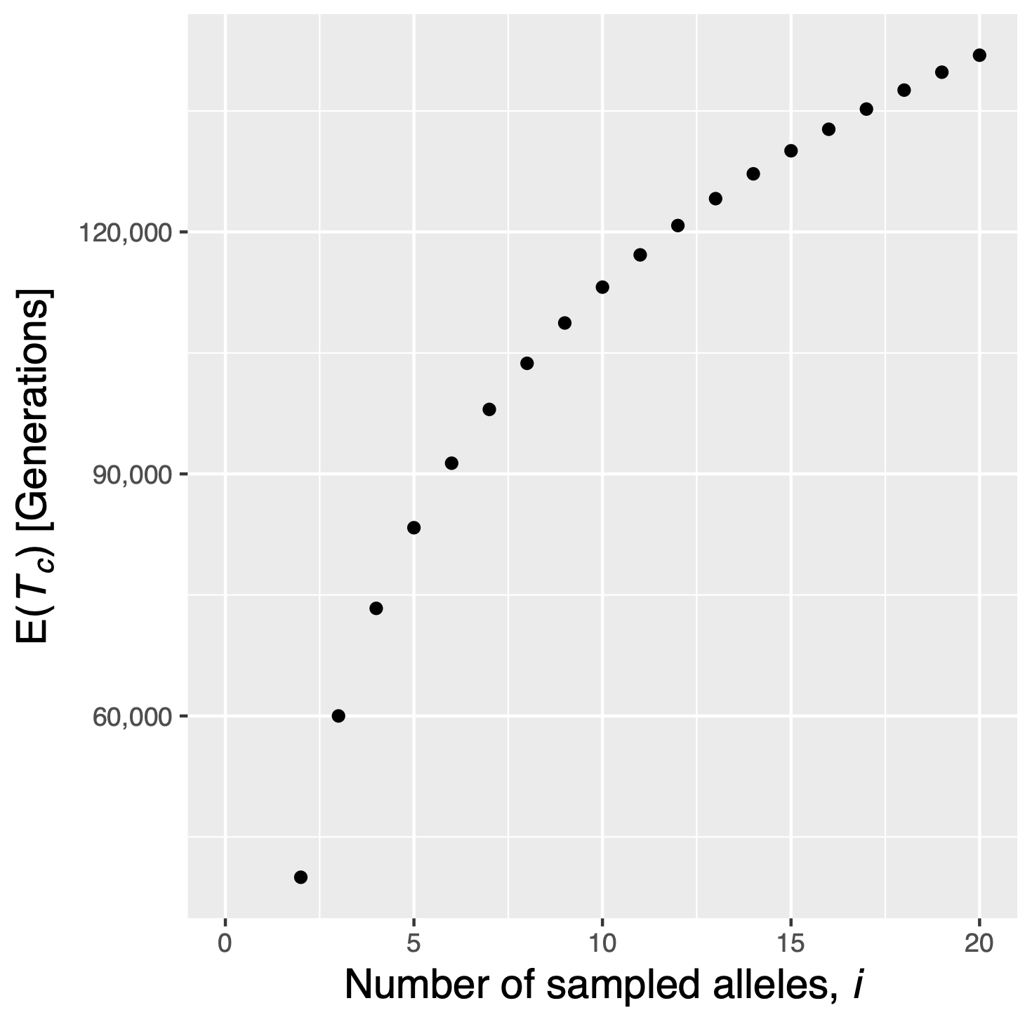
This result has important implications regarding the size of a sample: The total number of generations in a sample increases less with the sample size if $n>10$.

Calculation of the MRCA of a gene genealogy

By simplifying Equation $\text{(10)}$, it is possible to calculate the expected age of the deepest branch in a genealogy or the MRCA of the whole sample.

The average time for the coalescence of all alleles in a sample of size $n$ is $$\begin{array}{}\text{(11)}& E(T_C)=4N(1-\frac{1}{n})\end{array}$$ This allows to estimate how far it is possible to look back in time with a given sample size.

Mutations in the coalescent

Estimating the expected number of mutations

A large advantage of coalescent theory is the possibility to consider the genealogical process and the mutation process independently of each other because coalescent events occur separately from the occurrence of mutations. For this reason, the genealogical process is considered separately from the process that leads to genetic variation.

For the following discussion, we use an infinite sites model that assumes that each mutation affects a new site (i.e., nucleotide position) in the genome. Then, the expected number of polymorphic sites in a sample is the product of the mutation rate, $\mu$ and the total length of the gene genealogy of the sample.

This can be shown with a simple calculation in a sample of five alleles and a mutation rate of $\mu ={10}^{-4}$ mutations per generation in a gene. The first coalescence event that reduce the number of lines from five to four occurred on average 2,000 generations ago (Equation \eqref{tiderivation). At this point in time, five lineages exist (see Figure 9). For this reason, the number of generations in this section equals 10,000.

In the next section, there are four lines with a duration of 3,333 generations to the next coalescence events (4 $\times$ 3333 = 13,333 generations), then three lines for 6,666 generations (3 $\times$ 6,666 = 20,000 generations) and two lines for 20,000 generations (2 $\times$ 20,000 = 40,000 generations). This sums up the a total number of 83,333 generations or possibilities for mutations. By multiplying with a mutation rate of ${10}^{-4}$ mutations per generation we expect 8.33 neutral mutations distributed throughout the genealogy. It is important to note that this is an expectation value of a random variable.

Table 1: Total number of generations in the different section of the gene genealogy shown in Figure 9.

Coalescence time	Generations (approx.)
$T_5$	$5\times \mathrm{2,000}=\mathrm{10,000}$
$T_4$	$4\times \mathrm{3,333}=\mathrm{13,333}$
$T_3$	$3\times \mathrm{6,666}=\mathrm{20,000}$
$T_2$	$2\times \mathrm{20,000}=\mathrm{40,000}$
Total	$\mathrm{83,333}$

Estimating the expected numbers of segregating sites

By using Equation $\text{(10)}$ and remembering that $\theta =4N\mu$, the expected number of segregating positions in a sample of $n$ alleles can be estimated: $$\begin{array}{}\text{(12)}& E(S_n)=\mu E(T_c)=\theta \sum _{i=2}^n\frac{1}{i-1}\end{array}$$ By solving the equation for $\theta$ we obtain the following important result: $$\begin{array}{}\text{(13)}& \hat{\theta }=\frac{S_n}{1+\frac{1}{2}+\frac{1}{3}+\cdots +\frac{1}{n-1}}\end{array}$$

Equation $\text{(13)}$ can be used to estimate $\theta =4N\mu$ in a neutrally evolving population, if we know the sample size and the number of segregating polymorphisms of a population, i.e., by sequencing a locus in a sample of individuals.

This estimator corresponds to Nei’s estimator of nucleotide diversity, $\pi$, that we discussed earlier. Since the estimator in Equation $\text{(13)}$ has been formulated by Watterson, it is often called Watterson’s estimator, ${\theta }_W$ (Watterson, 1975).

It is also possible tocalculate the average number of polymorphism (i.e., nucleotide) differences of two randomly isolated alleles of a population. Equation $\text{(6)}$ describes the probability that two alleles from a population with a constant size had a common ancestor before exactly $t_n$ generations. The average time to coalescence of two randomly isolated alleles is $2\times 2N=4N_e$ generations (Figure 11).

Figure 11: Average time to coalescence of two randomly isolated alleles.

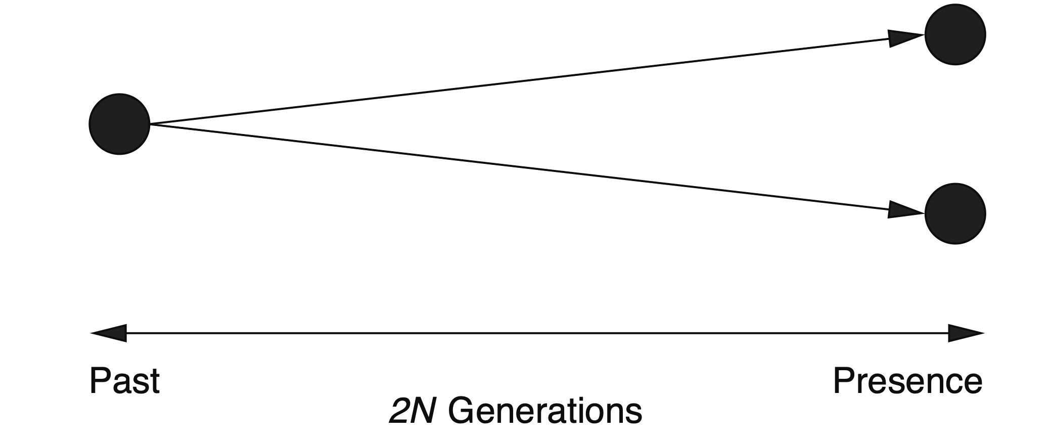
By adding the mutation rate $\mu$ (Mutations per nucleotide position per generation), the average number of differences $k$ between two alleles of length $m$ is then $$\begin{array}{}\text{(14)}& k=4N_e\mu m\end{array}$$

Problem: How to estimate $\mu$ and $N$?

So far, all parameters were expressed as abstract entities, or assumed to be known (e.g., $N$). In real populations, however, these quantities are unknown. It is important to note that in a coalescent with discrete generations, the genealogy does not depend onn the genealogical relations of unsampled alleles because they are not part of the sample, but on the total population size N which determines the genealogies of the whole population (i.e., the sampled and the unsampled population).

The parameter $N$ can be either the census or effective population size. The census size is the current size and the effective size is the size over evolutionary time. Both measures of $N$ are usually unknown. In the same manner, the mutation rate $\mu$ is usually unknown, but an independent estimate could be obtained from mutation accumulation experiments.

Two strategies are possible to deal with this situation:

1. Instead of trying to estimate an absolute value for a population size, all coalescent times are just expressed in units of 2N. Figure 9 shows that this is easily possible.
2. Estimate $\theta =4N\mu$ from the data without estimating the individual parameters $N$ and $\mu$.

We will not go into deeper analysis of these topics, as they are too advanced for the purpose of this topic.

Effects of population size change, population structure and selection on genealogies

Until now we made very strong assumptions on the process that did or did not occur. In biologically relevant populations, many of these assumptions are violated and we can ask ourselves, what the consequences are and how we can make use of the resulting changes. In the following, this weill be explained at a conceptual and not at a mathematical level.

Changes in population size

Historical changes in the population size are an important evolutionary process. If the population size increases, the probability of a coalescence event in recent generations is reduced. This causes longer terminal branches in the genealogies (Figure 12 B and C).

A population whose size decreased recently is characterized by short terminal branch lengths because the probability of coalescence events is larger with small population sizes.

Figure 12: A population with (a) a constant, (b) a strongly increasing and (c) an exponentially growing population size. Source: Unknown

An important effect of different population sizes is the distribution of polymorphisms on the individual evolutionary lineages. If a population is growing exponentially (think about the rapid geographic spread of a crop such after its domestication), the terminal branch lengths are very long and for this reason many mutations fall onto the terminal branches, which leads to an excess of rare mutations in the sample. For this reason, such a pattern supports the hypothesis of recent population growth if it is observed in numerous loci in a genome.

Population structure

If a population has been divided into different subpopulations with little gene flow between them, coalescence times should be short within subpopulations and large between subpopulations.

This results in a gene genealogy with short terminal branchaes and a long banch to the MRCA (Figure 13).

Figure 13: Effect of the presence of a population structure on the genealogy of a locus. label:fig:coalpopstructure

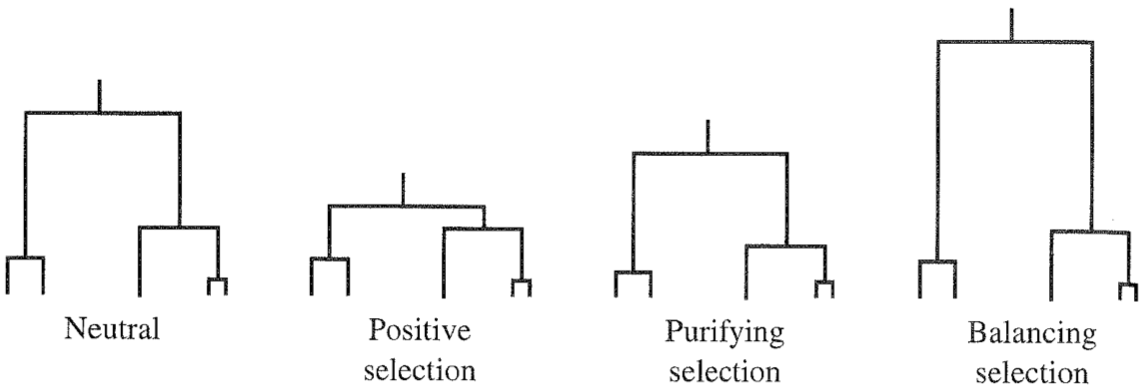
Natural and artificial selection

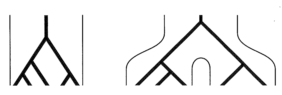
There are two major types of selection.

Positive or Darwinian selection:

This process increases the frequency of beneficial mutations in a population. With positive selection, certain alleles are transmitted into the next generation with a higher probability. The probability that two alleles originated from the same common ancestor is then increased. This causes shorter coalescence times and shorter times to the MRCA.

Negative or purifying selection:

This process causes the reduction of the frequency of disadvantageous or deleterious mutations. Under purifying selection, the probability that disadvantageous alleles are not transmitted into the next generation is increased, which also increased the probability of coalescence for the remaining alleles.

Both positive and purifying selection result in a decay of genetic variation and therefore cause shorter average coalescence times compared to neutral evolution (Figure 14).

Under balancing selection, two or more alleles are maintained in the population because they all are advantageous. These alleles independently acquired neutral mutations since their divergence and they are separated by long branches in a genealogy, which causes the a long time period until the MRCA of the complete sample is reached.

Figure 14: Randomly generated genealogies for different types of natural selection.

By walking along the genome and looking for regions with longer or higher level of polymorphisms (reflecting different times to the MRCA in different regionas), one can identify regions in which selection acted.

Recombination

Recombination causes that previously linked regions of a genome have different histories (i.e., genealogies). This is a significant complication of coalescence theory. However, it is possible to simulate genealogies with recombination, but it will not be discussed further here.

Why is coalescent theory useful?

Coalescent theroy is an explicit model of the genealogical tree of closely related alleles.

Different demographic histories (e.g. exponential growth) produce different tree likelihoods which result in different distributions of genetic diversity. A statistical inference of which demographic history shaped the observed diversity (e.g. one that most likely reproduces this diversity) is possible. For example, estimates of the growth rate of an exponentially growing population or a decision of whether there is any population growth are possible.

Tests of natural selection can be developed by scanning the genome for regions whose genetic diversity is significantly different from the best-fitting neutral model. Recombination can be modelled as well, for example by changing the genealogical tree across the genome.

Coalescent simulations

Coalescence theory can be used to simulate different evolutionary scenarios and to generate samples of alleles that are expected under this model. The coalescence process is probabilistic and it can be used to estimate random effects in the process.

The main use of coalescent theory is to simulate gene genealogies with mutations under different models of evolution and to compare simulated with observed genealogies or summary statistics like nucleotide diversity estimators, $\pi$ or ${\theta }_W$. Simulations are conducted as shown in Figure 15 and involve the following steps:

Figure 15: Outline of running and analysing coalescent simulations.

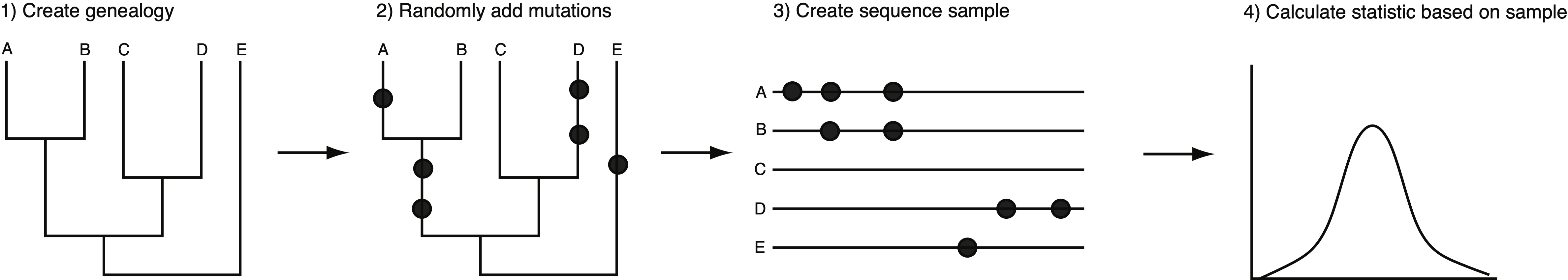
1. Create a random gene genealogy for a given sample size. The branch lengths are determined by the evolutionary model used. Different population histories produce different genealogies (see below).
2. Distribute random mutations on the genealogy. The probability of a mutation is determined by the mutation rate and the branch lengths of the genealogy. The probability of a mutation occuring on a particular branch is directly proportional to its length which is measured as numbers of generations.
3. Create a sample from the tree. A DNA sequence is generated for each individual in the sample. Depending on the program used, the location of the mutations are randomly distributed.
4. Calculate a test statistic from the simulated sample. Possible test statistics are nucleotide diversity or Tajima's $D$ (see below).
5. Repeat steps 1-4. In simulations these steps are repeated many times and generate a distribution of a test statistic such as nucleotide diversity for a given evolutionary model.

The implementation of coalescent simulations in computer programs has been described by Hudson (1990) and in subsequent papers. Since we are dealing with a random process, simulated genealogies differ from each other and it is necessary to simulate a large number of genealogies to make comparisons with observed data (Figure 16).

Figure 16: Tree genealogies resulting from coalescent simulations with the same parameter

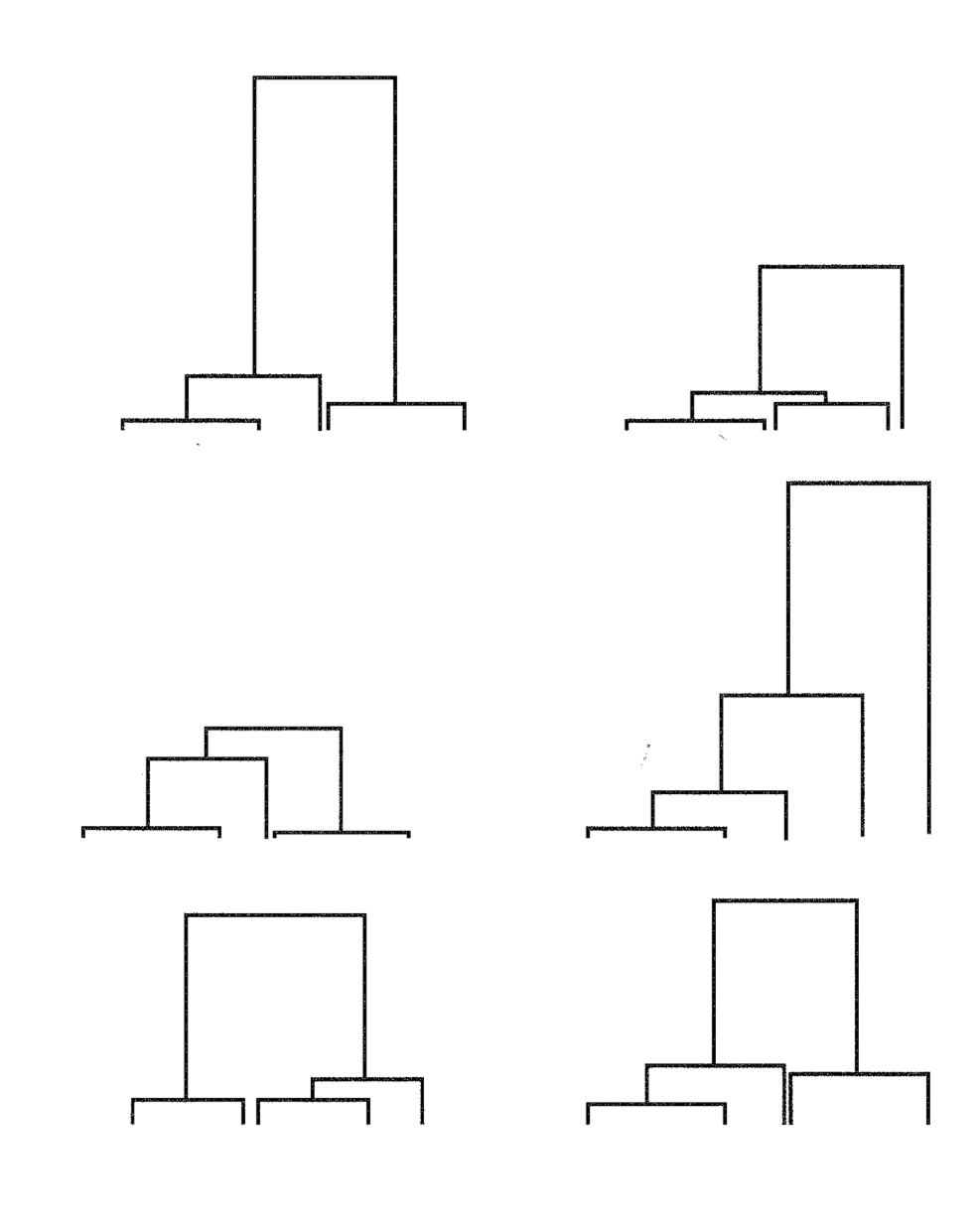
Genealogies of genes are influenced by the different evolutionary forces such as changes in population size, natural and artificial selection, the presence of a population structure and recombination.

These processes can be simulated and the resulting genealogies can be compared with observed genealogies to investigate which processes affected genetic variation at a locus.

Applications of the coalescent

Coalescent methods are increasingly used in the analysis of crop domestication and of selection during domestication. In the context of genetic resources and plant breeding numerous applications of coalescence theory can be envisioned:

Domestication history of a species

Coalescence theory can be used to compare different models of domestication, and to estimate when domestication occurred.

Allele mining

Based on a subsample from a gene bank, coalescent theory allows the estimation of the total number of alleles of a particular gene in a gene bank collection and can be used to predict how many accessions have to be characterized to identify, for example, 95% of the alleles segregating at a haplotype.

Definition of core collections

Core collections are sets of accessions that capture the maximal level of diversity of a sample with a certain number of individuals.

Detection of natural and artificial selection

Coalescent methods are useful to detect genes that evolved under selection in wild populations, during domestication, or in modern breeding programs.

Genetic relationship of heterotic pools

How are they defined and which exotic germplasm can we use to expand them?

Some of these applications will be elaborated in later lectures.

Key concepts

• Coalescence event
• Wright-Fisher model
  
• Gene genealogy
• Coalescent simulation
  
• Most recent common ancestor (MRCA)

Summary

• Coalescent theory is a method to investigate how evolutionary processes in the past have created patterns of genetic variation that we observe today.
• By using coalescent theory, many results of theoretical population genetics can be derived from basic statistical and genetic principles.
• Since the process of coalescence is independent of the mutation process, both processes can be modelled independently.
• Evolutionary processes such as selection and demographic changes change the shape of gene genealogies. These genealogies can be compared with expected neutral genealogies in tests of selection.
• Evolutionary processes like natural selection, population growth, population structure or recombination can be modeled with the coalescent by simulating the effect of these processes on branch lengths and the topology of simulated genealogies and by comparing them to observed genealogies.

Further reading

Each of the following chapters is a very good introduction into coalescence theory:

• Hartl and Clark, Principles of Population Genetics (4th Edition), Sinauer Associates (2007), Chapter 3.6 and 3.7
• Nielsen and Slatkin, An Introduction to Population Genetics - Theory and Applications, Sinauer Associates (2013), Chapter 3
• Matthew Hahn, Molecular Population Genetics, Sinauer Associates (2019), Chapter 6
• Asher Cutter, A Primer of Molecular Population Genetics. Oxford University Press (2019), Chapter 5.

There are two more advanced books on coalescent theory:

• J. Hein, M. H. Schierup and C. Wiuf: Gene Genealogies, Variation and Evolution - A Primer in Coalescent Theory. Oxford University Press (2005)
• John Wakeley: Coalescent Theory - An Introduction. Roberts and Company Publishers (2009)

Review articles and book chapters on coalescent theory in applications:

• Rosenberg and Nordborg (2002)
• Nordborg (2019)

Individual examples of applying coalescent theory to plant genetic resources will be provided in the following lectures.

Study questions

1. Describe the conceptual basis of coalescent theory. Which two processes are investigated separately?
2. What is the probability of a coalescence event in an random sample of two alleles in the previous generation?
3. How is the total length of a gene genealogy defined?
4. Explain how the number of expected mutations in a sample can be explained at a neutrally evolving locus can be explained with the help of coalescence theory.
5. What is the unit of time in coalescence theory and why is it chosen over other units of time? Is it possible to convert between units?
6. Why ist it sufficient according to coalescent theory to take a small sample of 10 - 20 individuals from a population to get a reasonable good estimate of genetic diversity estimates?
7. How do demographic processes such as an increase or a decrease of the population size affect the shape of genealogical trees?
8. Does the term most recent common ancestor (MRCA) apply to all individuals in the sample, or all individuals in a population from which a sample was taken?
9. What are potential applications of coalescence theory in the field of plant genetic resources?

Problems

Discussion questions

Which of the following statements are correct?

1. The waiting time for the next coalescence event in a sample increases the farther we go back in time.
2. The time to the most recent common ancestor decreases with increasing sample sizes.
3. The waiting time for the first coalescence event in a sample decreases with increasing sample size.
4. The total length of the coalescence decreases with increasing sample sizes.

Shapes of genealogies

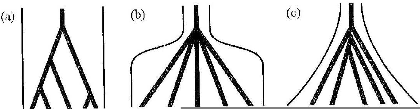
The following picture shows three different coalescence trees:

Figure 17: Different shapes of coalescent trees. Source: R. Nielsen and M. Slatkin /An Introduction to Population Genetics/ (Sinauer Associates. 2013)

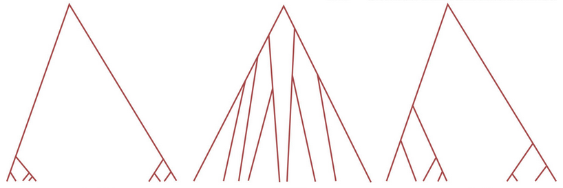
1. Compare the three coalescence trees. How do they differ?
2. Place randomly and evenly 10 mutations on each coalescence tree.
3. Compare the internal with the external branches of each coalescence tree. Where are more mutations?
4. Construct the unfolded site frequency spectrum for each coalescence tree.
5. Compare the three site frequency spectra. How do they differ?
6. Think about the three coalescence trees and their mutational patterns. Under which demographic scenario or type of selection would you expect each of the three coalescence trees?

Problems

Expected time to MRCA

In a sample of five alleles, what is the expected time to the most recent common ancestor under the standard coalescence model measured in $2N$ generations? What is the expected total tree length?

Expected numbers of segregating sites

A researcher sequences 5 diploid individuals (10 DNA sequences) from a population with an effective population size of 20,000 individuals. The total mutation rate for the regionn is 10^-5 per generation. Assuming a standard coalescence model and infinite sites mutation, how many segregating sites should the research expect to find in the data?

References

Hartl D, Clark A. 2007. Principles of population genetics, 4th ed. Sinauer Associates.

Hudson RR. 1990. Gene genealogies and the coalescent process. Oxford surveys in evolutionary biology 7:44.

Kingman J. 1982. The coalescent. Stochastic Processes and their Applications 13:235–248.

Maddison WP, Maddison DR. 1992. MacClade: Analysis of phylogeny and character evolution. Version 3. Sunderland: Sinauer Associates.

Nordborg M. 2019. Coalescent theory In: D. J. Balding IM, Marioni J, editors. Handbook of Statistical Genomics. John Wiley & Sons, Ltd. pp. 145–175.

Rosenberg NA, Nordborg M. 2002. Genealogical trees, coalescent theory and the analysis of genetic polymorphisms. Nat Rev Genet 3:380–390. doi:10.1038/nrg795

Watterson GA. 1975. On the number of segregating sites in genetical models without recombination. Theoret Pop Biol 7:256–276.