Analysis of genetic diversity
Module: Plant Genetic Resources (3502-470)
Motivation
Modern plant breeding programs follow a standard scheme in order to create improved varieties (Figure 1). Parents with favorable properties are crossed to generate new phenotypic variation and to combine favorable trait in single genotypes Among the offspring, favorable genotypes are selected and tested in muultiple environments to prove their value in comparison to existing varieties and the stability of their phenotype in different environments. The best performing genotypes are then registered as new varieties and marketed. These varieties are then again used as parents for novel breeding programs.
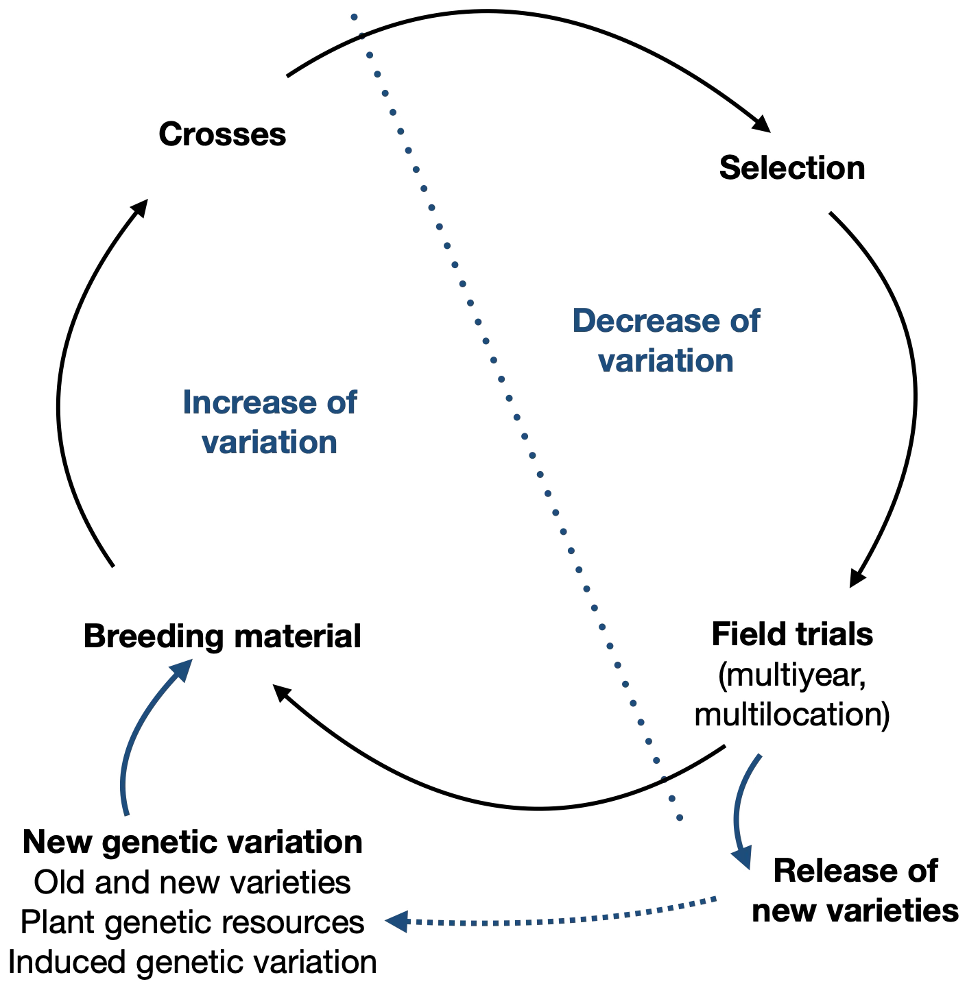
One consequence of breeding cycles is that at the beginning of the breeding program, genetic diversity is increased, and over time, genetic diversity is reduced because of selection and genetic drift. Furthermore, according to the DUS criteria, new varieties need to be distinct, uniform and stable for plant variety registration, i.e., a legal protection of the product of plant breeding. The uniformity requirement is responsible for the fact that with the exception of population varieties the vast majority of released varieties, in particular hybrid and line varieties are genetically homogeneous.
Over time, however, the available genetic diversity in a breeding population is reduced due to selection, and further breeding progress (also called genetic gain) becomes smaller and more difficult to achieve.
Learning goals
to be added
Variability of genetic diversity in breeding populations
Our motivation section showed that plant breeding strongly depends on the introduction of novel genetic variation from genetic resources. This leads to the question, which type and how much new genetic variation is optimal for sustaining long term breeding progress to produce productive, healthy and adapted varieties.
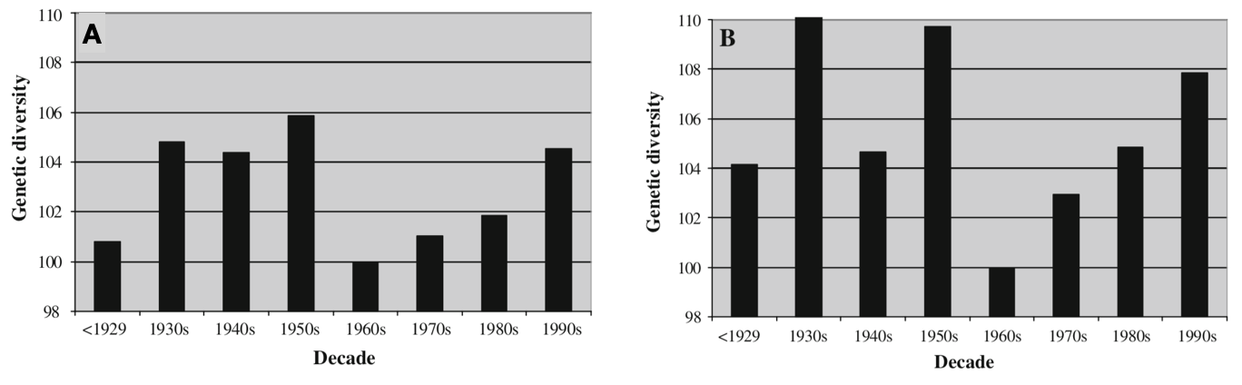
The effect of repeated breeding cycles is seen in Figure 2 diversity. It shows the results of a metastudy on the genetic diversity of varieties of various field crops (wheat, maize, barley, oat, flax, pea, rice, soybean) that were released in the 20th century in different regions of the world. The regional genetic diversity of varieties (i.e., Europe or North America) was assessed with molecular markers. Both the analysis of the complete dataset of 44 individual studies and of a subset of 20 studies of wheat indicate a drop in diversity in the 1960s after a period of substantial diversity. Starting from the 1970s, plant breeders managed to increase the diversity by introgression of new genetic diversity with the result that no substantial reduction in the regional diversity has taken place.
It should be noted, however, that this analysis is based on a fairly small numbers of molecular markers per species and that errer margins tend to be large with respect to the estimates.
The paradox of genetic diversity
Based on the knowledge of Mendelian inheritance and of genetic diversity one may ask, why new genetic diversity needs to be introgressed in plant breeding programs if the interplay of existing diversity and recombination are able to produce potentially unlimited amounts of diversity? This discrepancy between observed and expected diversity is the paradox of genetic diversity and explained in the following.
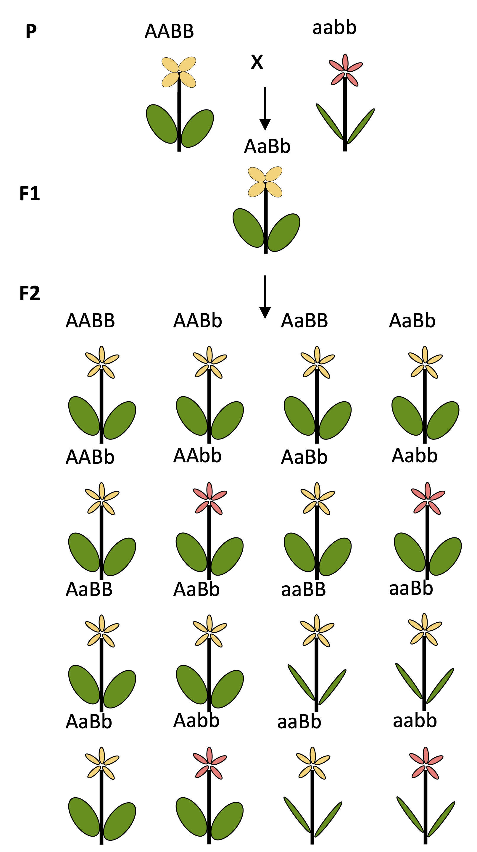
Figure 3 shows a cross of two parents, which are homozygous for two genes. The two parents differ at the two alleles from each other. The F1 generation is heterozygous, and in the F2 generation the alleles start to segregate according to Mendel’s rules.
We assume that the two genes control two different traits (flower color and leaf shape). From this follows that the number of possible combinations of the two traits is \(3^2=9\) genotypes.
Now we assume that the two parents differ at 21 loci. Again the F1 individuals are heterozygous for all loci, but they start to segregate in the F2 generation. Based on the number of genotypes, there are more than 10 billion (\(10^{9}\)) possible genotypes. Under the assumption that each locus controls a different trait, there are the same number of potentially different phenotypes. These are many more phenotypic variants originating from a single cross than a breeder can handle in a breeding program.
| \(P_{1}\) | AABBCCDDEEFFGGHHIIJJKKLLMMNNOOPPQQRRSSTTUU |
| \[\times\] | |
| \(P_{2}\) | aabbccddeeffgghhiijjkkllmmnnooppqqrrssttuu |
| \[\Downarrow\] | |
| \(F1\) | AaBbCcDdEeFfGgHhIiJjKkLlMmNnOoPpQqRrSsTtUu |
| \[\Downarrow\] | |
| \(F2\) | \(3^{21} = 10,460,353,203\) genotypes |
What then is the paradox of genetic diversity? While it is easy to generate novel phenotypic variation by combining different alleles of different genes in the offspring of a cross, there is often not sufficient useful variation for traits that need to be improved available in breeding populations.
In other words, there may not be enough genetic variation at genes involving 21 different traits within a breeding population even though it would be easy to generate new genetic diversity (i.e., combinations of different phenotypes) by crossing.
For this reason, new genetic variation needs to be identified, crossed with existing material and evaluated on a phenotypic level in so-called prebreeding programs to increase phenotypic diversity by introgressing new genetic diversity.
Loss of genetic variation due to breeding
There are several reasons why breeding populations are impoverished for genetic variation in useful traits. Possible reasons are:
- Bottlenecks
- Only a small proportion of total genetic variation is included in a breeding population. The establishment of a new population by selecting a small number of funders from the ancestral population is also called founder effect. The new population likely has a much smaller level of genetic variation and a very different frequency of alleles.
- Genetic drift
- Random fixation of alleles, especially profound in small populations.
- Selection
- Fixation of advantageous alleles or loss of disadvantageous by selection.
For an explanation of how these processes reduce genetic variation, you may consult introductory population genetics textbooks.
The reduction of genetic diversity occurred primarily at two stages during the history of crop plants. These are the domestication of a crop from its wild ancestor, and modern breeding programs that apply strong selection to breeding populations. The two stages can be compared to a funnel that represent a genetic bottleneck (Figure 4).
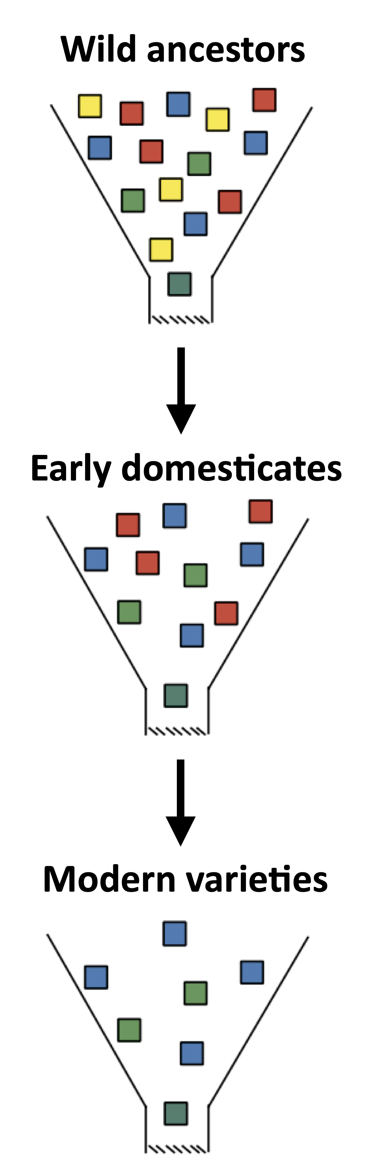
In the discussion of genetic erosion of crop species, Figure 4 has become iconic, and measures of genetic diversity of crop plants and their wild ancestors confirm this notion. However, this figure is too simplistic because in many crops that were domesticated thousands of years ago, new genetic diversity originated by mutation, which may have been advantageous for cultivation and was selected by farmers and early breeders. There is surprisingly little research in this direction and the narrative of a loss of genetic variation prevails.
Genetic vulnerability due to a narrow genetic basis
Populations that lack genetic variation are called vulnerable because they either suffer from inbreeding depression (in outbreeding species like maize) or have little genetic variation at resistance genes, which makes it easy for pathogens to spread in a population, once they overcome resistance mechanisms.
Two historical examples:
- Potato leaf blight in Ireland (1845-1849)
- It was caused by the pathogen Phytophtora infestans. As a result one million people starved to death and one million people emigrated to the US.
- Southern leaf blight epidemics in the Southern US (1970)
- Maize varieties with the so-called texas-T cytoplasm were wiped out by Southern leaf blight. The epidemics resulted in a harvest loss in this year. Although the economic damage was limited, this epidemic epidemic raised awareness of genetic vulnerability.
An important consequence of genetic vulnerability is the high cost required for fungicides to keep pesticides under control in modern large-scale farming systems.
The Southern leaf blight epidemic had a relatively small (economic) impact, but the Great Famine that was caused by potato leaf blight had major historical consequences (Zadoks, 2008).
A lack of genetic diversity of potatos allowed a single strain of the pathogen P. infestans to produce the epidemic. At that time a single variety of potato was planted, which was favored by the fact that it can be clonally propagated and produces genetically identical offspring.1
1 For a very short summary, see here
The genomic analysis of a herbarium strain of P. infestans showed that a single strain originating from Mexico was causing the epidemic, which today has been replaced by other strains (Birch and Cooke, 2013; Goss et al., 2014; Yoshida et al., 2013).
Genetic vulnerability and genetic erosion
In the context of crop genetic diversity, two terms are frequently used.2
2 See, for example, FAO (2010)
Genetic vulnerability results if a widely planted crop is uniformly susceptible to a pest, pathogen or environmental hazard as a result of its genetic constitution, thereby creating the potential for widespread crop losses.
Genetic erosion is the loss of individual genes and the loss of particular combinations of genes (i.e. of gene complexes) such as those maintained in locally adapted landraces.
There are alternative uses of the term ‘genetic erosion’ (Khoury et al., 2022):
- Loss of old varieties or landraces of a given crop
- Loss of (useful) genes or alleles present in a crop species, landrace, variety
Types of genetic variation
If the genetic diversity in a breeding population or a crop species in general is limited, it is necessary to search for new variation, such as in old varieties or in wild relatives.
However, genetic diversity is not useful per se, and it is necessary to differentiate among different types of genetic variation.
One may differentiate the total genetic variation into three major types of genetic variation:
Useful genetic variation influences traits that are selected during breeding in a positive manner. Such variation is expected in the following classes of genes:
-   Yield genes
-   Adaptation genes
-   Resistance genes
-   etc.
Neutral genetic variation is the fraction of genetic variation without phenotypic effects. Since it is not selected, it mainly evolves under genetic drift (i.e., random evolution) in a population.
Deleterious genetic variation is any genetic variation that reduces the favorable traits of a crop such as the yield or quality of the crop harvest. If it can be recognized as such by the breeder, it is removed by selection during the breeding process.
There is a large body of theory and also empirical studies in population genetics on the question which proportion of variation segregating in populations belongs to each of these three classes, and which methods are suitable to classify genetic variants into these classes3
3 See, for example, our work on deleterious mutations segregating in wild and crop plants (Günther and Schmid, 2010).
What are plant genetic resources (PGR)?
To introduce the topic of genetic diversity in the context of PGR, we first define plant genetic resources and then show why new genetic diversity in form of PGR are important and required in the context of the paradox of genetic diversity discussed above.
The 4th international technical conference of FAO on PGR in Leipzig 1996 used the following definition for plant genetic resources4:
4 See the report on the conference: Link.
… generatively or vegetatively reproducible material of plant of current or potential value, including landraces, related wild sprecies and wild forms and special genetic material of crop plants
A much simpler definition was given by Pflanzenzüchtung (1993):
… the complete genetic material that is available for breeding of a crop plant.
In the age of genetic engineering and synthetic biology, we can even further broader expand this definition to
any genetic material and variants that is naturally available or can be artificially generated and used in plant breeding.
Sources of new genetic variation
If genetic diversity (e.g., in a given crop species) is limited, there are several sources to utilize new genetic variation. The sources include
- New and minor crops (Neodomestication)
- Close relatives of crops (Neodomestication, Redomestication, Introgression)
- Wild ancestors of crop species
- Land races and traditional cultivars
- Modern elite varieties of different geographic origin
- Induced mutations by chemical (Mutagens), physical (Irradiation) or biological (Genome editing) treatments
In the breeding of commercial varieties, the released varieties of competitors (if they are not patented) likely are the main sources of new genetic variation. This is possible because of the breeder’s exemption granted by plant variety protection laws in many countries and also a meaningful approach because released commercial varieties are usually purged of much deleterious variation that frequently segregates in traditional cultivars that have not been improved by breeding (Figure 5).
Crop gene pools as sources of new genetic diversity
In an effort to have a more rational and systematic access to new genetic diversity for crop plants, Harlan and de Wet developed the concept of crop gene pools Harlan and Wet (1971). Essentially, for each crop several gene pools are defined that describe the genetic and taxonomic relationship to a given crop plant (Figure 6).
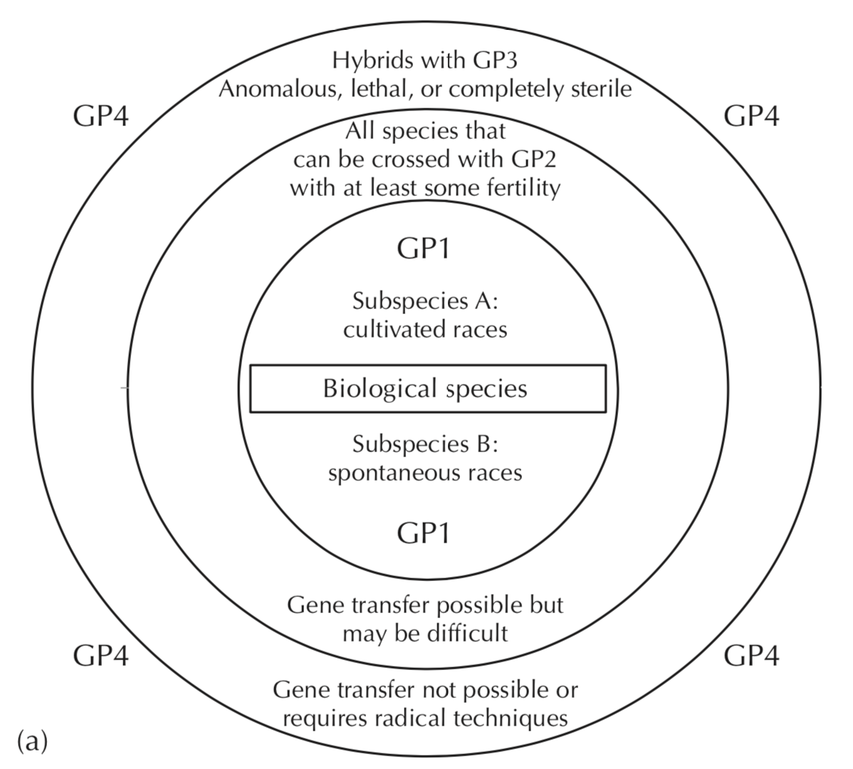
According to this definition, there are four gene pools:
- Gene pool 1 (GP1):
- This pool is defined by the biological species concept, which states that all genotypes that can be crossed with each other and form fertile offspring belong to the same species. Therefore, this GP1 includes usually the ancestors of crops as well as all subspecies of a species that may reflect either cultivated types or spontaneous types that are phenotypically variable.
- Gene pool 2 (GP2):
- It includes closely related species that can be successfully crossed with the crop species, but produce offspring with limited viability or limited fertility indicated by partial sterility. This pool frequently include close relatives that my harbor interesting disease resistance genes. Taxonomically such species may be other species in the genus.
- Gene pool 3 (GP3):
- This gene pool includes more distantly related species. Crosses with the crop species may produce offspring, but it either has an anomalous phenotype, or the embryo does not develop into an adult plant because of lethality or are completely sterile. Quite frequently these barriers to producing offspring can be overcome by biotechnological treatments in order to produce offspring that can be included in further breeding processes.
- Gene pool 4 (GP4):
- It includes all other species where crosses with the crop species are not successful.
The first three gene pools an be utilized by classical breeding or biotechnological approaches such tissue culture or protoplast fusion. The fourth gene pool includes species that can not be crossed to a given crop but may provide useful genes that can be introduced into the crop by genetic engineering.
In the following, the concept of gene pools as sources of novel and useful genetic diversity is demonstrated for canola, Brassica napus.
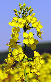
The primary gene pool consists of
- Modern elite varieties of canola (Brassica napus)
- Landraces and traditional cultivars
- German Brassica napus (rapeseed) (Wikipedia)
The secondary gene pool includes
- Brassica rapa (Turnip; several subspecies used as vegetables) (Wikipedia)
- Brassica oleracea (Cabbage and derived vegetables) (Wikipedia)
- Brassica nigra (Black mustard) (Wikipedia)
The four Brassica species have a special chromosomal relationship that is called ‘Triangle of U’, which essentially states that the genomes of three ancestral species merged to form the genomes of several modern Brassica vegetables (Wikipedia) see also the lecture or gene flow).
The four species can be crossed with each other relatively easily and produce F1 hybrids (Hauser et al., 1998).
The tertiary gene pool includes
- Raphanus (Radish) (Wikipedia)
- Crambe (Sea kale; Meerkohl) (Wikipedia)
- Arabidopsis (thale cress) (Wikipedia)
Somatic cell lines between Arabidopsis thaliana and Brassica nigra could be produced by protoplast fusion (Siemens and Sacristán, 1995), which demonstrates that genes can be transferred between the two species. However, further complications may arise by the fact that the chromosomes between the two species may not recombine because of extensive sequence differences.
Key questions in the context of PGR
Based on the above considerations, several questions arise with respect to the level and use of genetic diversity in plant genetic resources and their use in breeding:
- What is the level of genetic diversity within and between modern elite breeding populations?
- Does ‘exotic’ breeding material have a higher level of genetic variation that can be introgressed into modern varieties?
- What type of genetic diversity is useful or deleterious?
- How can useful genetic variation be identified?
Much contemporary research on genetic resources is focused on answering these questions.
An example of a successful introduction of new variation
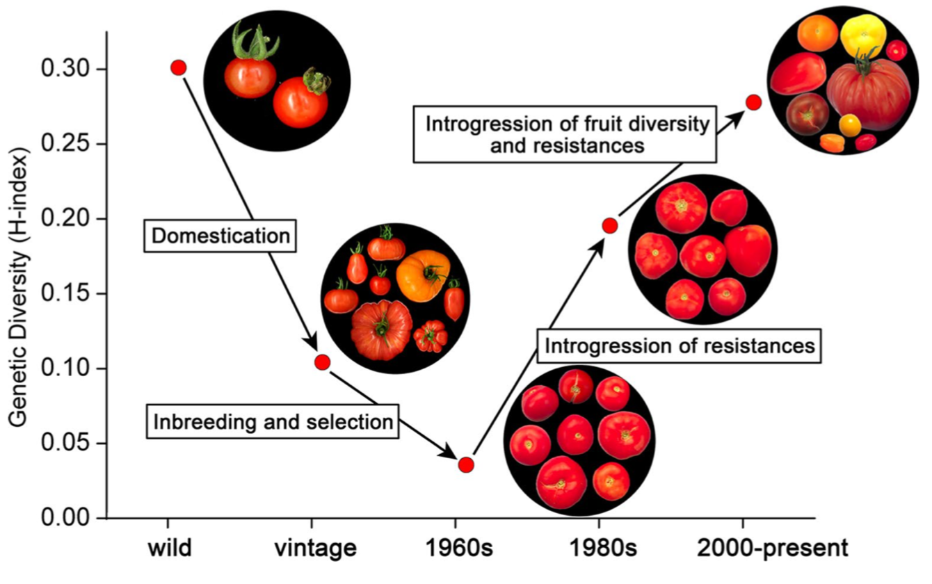
The effect of a loss in genetic diversity and subsequent gain by intregression of plant genetic resources can be demonstrated with the breeding history of tomato in the Netherlands (Schouten et al., 2019). The wild ancestors of cultivated tomato are Solanum lycopersicum var. lycopersicum, S. lycopersicum var. cerasiforme, and S. pimpinellifolium. From these ancestors, heirloom types and landraces originated by domestication processes. Inbreeding and selection among these old (vintage) varieties led to commercial varieties in the 1960s with a very low genetic and phenotypic diversity. During this time Dutch tomatoes developed a reputation for being tasteless and watery, which led to the “waterbomb” (in German: “Wasserbombe”) crisis. Breeders reacted and introduced more exotic genetic variation into the breeding material to increase multiple aspect that include taste, shape and diesease resistances. From the 1970s onwards, resistances to diseases and pests were introgressed from distant species, including S. peruvianum, S. pennellii, S. chilense, and S. habrochaites, increasing genetic diversity among commercial tomato varieties considerably. After the 1980s, fruit size, color, and flavor started to vary substantially, further increasing the genetic diversity of modern varieties.
As a result, the genetic diversity of Dutch tomato varieties increased. The temporal dynamics is shown in Figure 8 and the data are based on genotyping 90 varieties using a SNP array and calculating Nei’s index \(H\) for genetic diversity, which will be introduced below.
Quantification of genetic variation
In current studies of genetic variation, essentially two types of data are used: Genetic markers such as single nucleotide polymorphisms (SNPs), and DNA sequences. Markers target individual polymorphisms with a known location in a genome using a experimental assay, whereas DNA sequences analyse the complete set of polymorphisms in a genomic region or even the whole genome. To derive the theory for quantification of genetic variation, we first focus on SNPs, i.e. individual genetic polymorphisms.
We first introduce the following conventions: A locus is indicated with a capital letter. \(A\), \(B\), etc. are different markers (e.g., SNPs) with the alleles \(A_1\), \(A_2\), etc.
The relative frequency of allele \(A_1\) is \(p\), and of allele \(A_2\) is \(q\).
If there are more than two alleles, frequencies are expressed as \(p_1,p_2,p_3,...\)
There are three genotypes in a population of diploid organisms: two homoygous marker genotypes \(A_1A_1\) and \(A_2A_2\), and the heterozygous genotype \(A_1A_2\).
The relative frequencies in the populations are written as \(x_{ij}\):
| Genotype: | \(A_1A_1\) | \(A_1A_2\) | \(A_2A_2\) |
| Relative frequency: | \(x_{11}\) | \(x_{12}\) | \(x_{22}\) |
The sum of relative frequencies is 1: \[\begin{equation} x_{11} + x_{12} + x_{22} = 1 \end{equation}\]
From genotype frequencies, the allele frequencies can be calculated directly. The frequency \(p\) of allele \(A_1\) is \[\begin{equation} \label{allelefreq} p = x_{11} + \frac{1}{2}x_{12}, \end{equation}\] and the frequency \(q\) of allele \(A_2\) is \[\begin{equation} \label{allelefreq2} q = 1 - p = x_{22} + \frac{1}{2}x_{12}. \end{equation}\]
Some markers or marker types (such as simple sequence repeats, SSRs) have more than two alleles, but the calculation of relative allele frequencies is straightforward.
For a marker with \(n\) alleles we write
| Alleles: | \(A_1\) | \(A_2\) | \(A_i\) | \(A_j\) | \(A_n\) |
| Frequencies: | \(p_1\) | \(p_2\) | \(p_i\) | \(p_j\) | \(p_n\) |
Indices \(i\) and \(j\) indicate different alleles, and \(x_{ij}\) gives the frequency of genotype \(A_iA_j\).
Under the assumption that in heterozygotes \(i \ne j\) and, as a convention, \(i < j\), we obtain a total frequency of 1 when summed over the frequencies of all alleles.
With \(n\) alleles segregating at a locus we write \[\begin{equation} \label{multifreq} x_{11} + x_{22} + \cdots + x_{nn} + x_{12} + x_{13} + \cdots + x_{(n-1)n} = \sum_{i=1}^{n}\sum_{j \ge 1}^{n}x_{ij} = 1. \end{equation}\] Another measure of genetic variation is Nei's gene diversity,\(H\), which is an estimator of the average observed heterozygosity of markers (Nei, 1973).
It is essentially an estimate that two randomly chosen alleles in a population are not identical, and is calculated for a single marker as \[\begin{equation} \label{nei} H = 1 - \sum_{i=1}^np_i^2 \end{equation}\] where \(n\) is the number of alleles of a marker and \(p_i\) is the observed frequency of allele \(i\). An unbiased estimator is given by \[\begin{equation} \label{neiunbiased} \hat{H}=\frac{n}{n-1}(1 - \sum_{i=1}^np_i^2). \end{equation}\] Gene diversity is the most widely used measure of genetic variation of markers, because it is easy to calculate and it can be used for biallelic and multiallelic markers.
A related measure is polymorphism information content (PIC), which was originally introduced for use in human genetics (Botstein et al., 1980).
It refers to the value of a marker for detecting polymorphism within a population, depending on the number of detectable alleles and the distribution of their frequency for a given marker.
A measure on informativeness is highly useful in selecting parents for genetic mapping because one wants to maximize the chance that a set of markers has a high power to detect a quantitative trait locus (QTL) in a genetic mapping study because they have a high chance of being polymorphic among offspring as they are likely different between the parents.
For outbred and heterozygous individuals, the PIC value of a marker is defined as \[\begin{equation} \label{pic} \text{PIC} = 1-\sum_{i=1}^np_i^2-\sum_{i=1}^{n-1}\sum_{j=i+1}^n2p_i^2p_j^2, \end{equation}\] $$ where \(n\) is the total number of alleles of a locus, and \(p_i\) and \(p_j\) the frequencies of alleles \(i\) and \(j\), respectively.
The occurrence of rare alleles has less impact on the PIC than alleles occurring with high frequencies.
A simplified version was developed assuming that the inbred individuals selected for mapping are homozygous (Anderson et al., 1993).
Then, the PIC of a marker \(i\) is: \[\begin{equation} \label{pic2} \text{PIC}_i = 1 - \sum_{j-i}^np_{ij}^2, \end{equation}\] where \(p_{ij}\) is the frequency of the \(j\)-th pattern for marker \(i\) and the summation extends over \(n\) patterns.
Note that this measure corresponds to Nei’s gene diversity measurement.
The PIC for multiple markers can be calculated by taking the average of PIC values of each marker.
Depending on the type of mapping study, PIC values can be used to select markers for genotyping or individuals for creating a mapping population. Therefore, this measure is frequently used in the design of genotyping arrays in breeding programs.
Quantification of DNA sequence variation
In comparison to SNP markers, DNA sequencing identifies all polymorphisms of a locus, and one obtains a group of coupled markers.
The different combinations of alleles of different polymorphisms on the chromosome, in a genomic region or in a gene are called haplotypes.
The following sequence alignment shows the hypothetical DNA sequence of a short region of 10 base pairs from two outbred, heterozygous, diploid individuals.
                A)            B)
Position        1234567890    1234567890
Individual 1    GATCGAACAG    G.T......G
Individual 1    GAACGAACAT    G.A......T
Individual 2    TATCGAACAG    T.T......G
Individual 2    TATCGAACAG    T.T......G
The difference between A) and B) is that in the latter, only the variable positions in the sequence alignments are shown with letters and invariable sites with dots.
In this sample, three single-nucleotide polymorphisms are observed and three haplotypes (i.e. combinations of polymorphisms). Individual 2 is homozygous at this region, because both sequences are identical (they are the same haplotype). Using this sequence alignment, several descriptive statistics can be calculated.
If each sequence differs from each other one (given that the sequenced region is long enough), heterozygosity as a measure of genetic variation becomes obsolete because nearly each individual is heterozygous.
Instead, a new measure is defined, which is called nucleotide polymorphism.
It describes the proportion of nucleotide positions in a sample that are polymorphic and is calculated as \[\begin{equation} \label{nucpoleq} P_n = \frac{n_P}{n_t} \end{equation}\] with \(n_P\) as the number of polymorphic nucleotide positions and \(n_t\) as the total number of sequenced nucleotide polymorphisms in the sequenced region.
In the above sequence alignment, \(P_n=3/10=0.3\).
A second, and more widely used measure for DNA sequence variation is nucleotide diversity, \(\pi\).
It is defined as average pairwise nucleotide difference and can be calculated as \[\begin{equation} \label{nucdiveq} \pi = \frac{1}{n}\sum_{i=1}^n \sum_{j=i+1}^np_{ij}, \end{equation}\] where \(p_{ij}\) is the proportion of nucleotide differences between allele \(i\) and \(j\) of a sample of \(n\) alleles. For example, if two alleles differ at 3 of 10 nucleotide positions, \(p_{ij}=0.3\).
This measure describes the average proportion of nucleotide positions, which are polymorphic (i.e., different) between any to randomly chosen alleles of a locus in a population.
A more efficient calculation of nucleotide diversity is achieved by first counting the number of haplotypes and the differences between the different haplotypes. If \(\pi_{ij}\) is the proportion of nucleotide differences between haplotypes \(i\) and \(j\), and \(p_i\) and \(p_j\) are the relative frequencies of each of the two haplotypes, then nucleotide diversity is calculated in a sample with \(k\) distinct haplotypes as \[\begin{equation} \label{hapdiv} \pi = \sum_{i=1}^{k}\sum_{j=1}^{k}p_ip_j\pi_{ij} \end{equation}\] Yet another simple method to calculate nucleotide diversity to calculate \(\pi\) is given in the following 5
5 The method is taken from Hartl and Clark (2007), p. 34 f
- Calculate average number of pairwise mismatches between haplotypes
- Count number of mismatches for every pair of aligned sequences
- For \(n\) sequences, there are \(n(n-1)/2\) possible pairs of sequences
- Calculate \(\Pi\): \(\Pi = \frac{\text{Total number of nucleotide mismatches}}{\text{Total number of pairwise comparisons}}\)
- Calculate on a per-nucleotide basis genes of different length: \(\pi = \frac{\Pi}{L}\) where \(L\) is the length of the alignment in nucleotides
This value of \(\pi\) describes the nucleotide diversity of a population. However, it is biased and can not be used directly as an estimator for population parameter using a sample.
Nei (1987) proposed a simple correction that results in an unbiased estimator and is calculated as \[\begin{equation} \label{neiunb} \pi = \frac{n}{n-1}\sum_{i=1}^{k}\sum_{j=1}^{k}p_ip_j\pi_{ij} \end{equation}\]
Both statistics have in common that they can be used to estimate a very important parameter of populations, namely \(\theta=4N_e\mu\), where \(N_e\) is the effective population size and \(\mu\) the mutation rate, expressed as number of mutations per nucleotide per generation. The parameter \(\theta\) is often called the population mutation parameter and describes the expected level of genetic diversity in equilibrium populations, in which the processes of mutation and genetic drift are in an equilibrium.6
6 :Consult introductory population textbooks for an explanation.
It should be noted however, that nucleotide polymorphism, \(P_n\), needs to be modified to be an estimator of \(\theta\) as \[\begin{equation} \label{nucpol} \hat{\theta_W} = \frac{P_n}{a_n}, \end{equation}\] where the factor \(a_n\) is \[\begin{equation} \label{corrfac} a_n = \sum_{i=1}^{n-1}\frac{1}{i}. \end{equation}\]
The variable \(\theta_W\) stands for Watterson’s \(\theta\) (Watterson, 1975) who showed that it is an estimator of \(\theta=4N_e\mu\). If nucleotide diversity is used as an estimator of \(\theta\) it is often designated as \(\hat{\theta}_{\pi}\).
Both \(\pi\) and \(\theta_{W}\) have the characteristics that they are unbiased estimators of the population mutation parameter, \(\theta = 4N_{e}\mu\) in populations that evolve without selection. If the the mutation rate is known, they can be used, for example, to estimate the effective population size in populations.
There are other statistics that can be used to describe genetic variation in sequencing data. They include haplotype diversity and the mismatch distribution. For example, the haplotype diversity is calculated as \[\begin{equation} \label{hapdiv} h = \frac{n}{n-1}(1-\sum_{i=1}^n x_i^2) \end{equation}\] where \(x_i\) is the frequency of haplotype \(i\) and \(n\) is the number of different haplotypes. Frequently, these estimators are highly correlated, because they measure similar properties of the data.
In most studies of crop genetic diversity that use sequences, nucleotide diversity, \(\pi\), is used as measure of genetic diversity.
Limitations of current estimators of genetic diversity
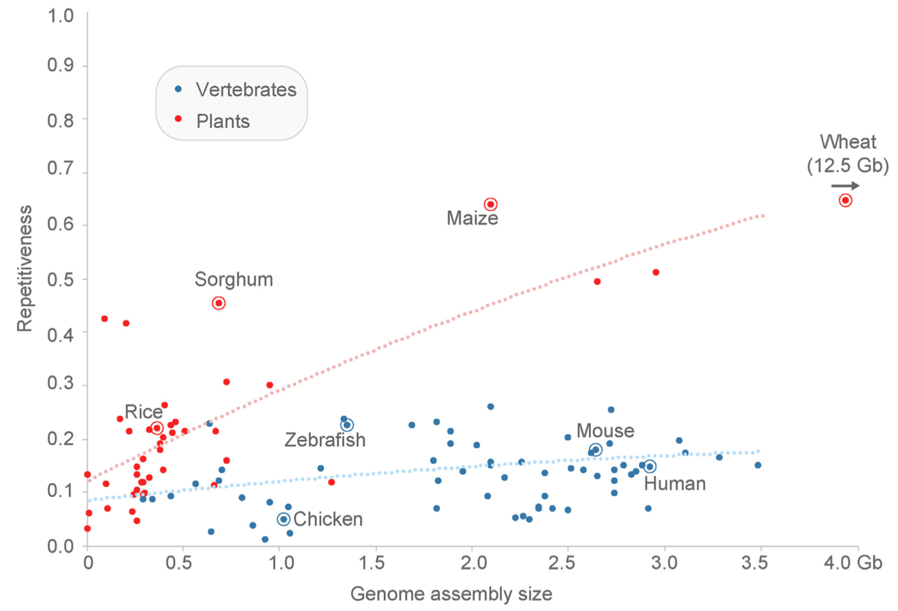
The sequencing of complete plant genomes and the resequencing of the genome sequences of multiple individuals revealed that very complex types of genomic polymorphisms segregate in plant populations. They result from insertions and deletions of DNA, from the activity of transposable elements (TEs) and from gene duplications, which creates many repetitive regions in plant genomes. For this reason, plant genomes tend to be much more repetitive than animal genomes (Figure 9).
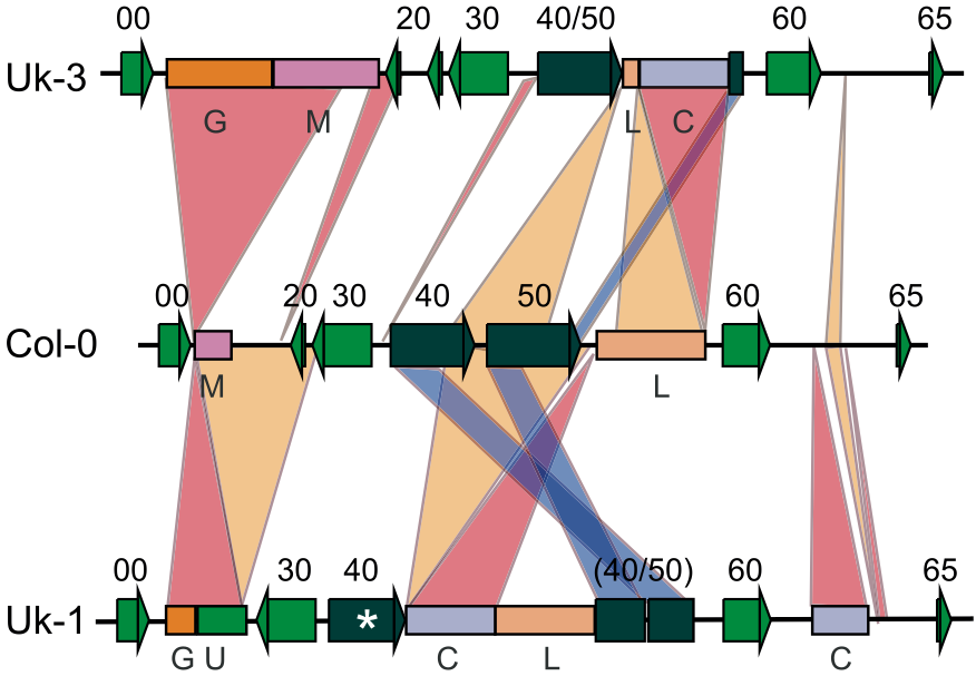
As an example, a genomic region of the model plant Arabidopsis thaliana, which was sequenced a high quality in three individuals collected at different locations of the species distribution range and in which all genes (and gene fragments) were annotated shows the complexity of rearrangments (Figure 10). As consequence of these rearrangments, no simple multiple alignment to calculate nucleotide diversity measures discussed above is possible, and new measures of describing genetic diversity have to be developed.
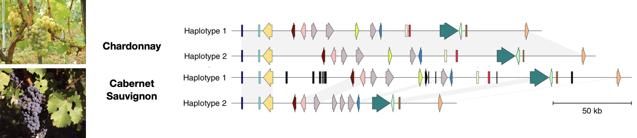
Similar rearrangements are observed in crop species such as grapevine Vinis vitifera or maize. For example, Figure 11 shows the schematic alignment of a genomic region from Chardonnay and Caubernet Sauvignon. The alignment shows a high degree of genetic differentiation caused by presence and absence of genes between the two haplotypes of each of the two varieties, and in addition of the two varieties. In total, the two varieties differ by a total of 2,217 genes (6% of all genes), which are present or absent in one of the two varieties relative to the other.
In summary, these comparisons show that complex polymorphisms result from different and interaction types of mutations like point mutations, insertions/deletions and rearrangements and transposon insertions. Such polymorphisms can not be described with the simple, nucleotide-based measures of genetic differentiation. Unfortunately, no suitable statistics have been developed yet to quantify this type of genetic variation, but there developments to model diversity of these complex variants that are either based on \(k\)-mers (sequence words) or genome graphs.
Key concepts
Summary
- Nowadays, DNA-based markers such as single nucleotide polymorphisms and DNA sequences are the method of choice for analysing genetic variation.
- Plant breeding depletes genetic variation over time and leads to a slowdown of genetic gain per time.
- Genetic resources are genetic material available for breeding, which increases genetic diversity in breeding pools or breeding programs.
- The gene pool concept describes the relationship between a crop species and its genetic resources.
- The quantification of genetic variation differentiates between allele and genotype frequencies.
- The number of polymorphic loci (polymorphism) and the heterozygosity are used as measures to estimate and compare levels of genetic variation in population.
- Marker- and sequence-based estimates of DNA variation are derived from polymorphism and heterozygosity.
- For markers, the most important estimate of diversity is gene diversity, \(H\), and for DNA sequences, nucleotide diversity, \(\pi\) and Watterson's \(\theta_{W}\), which are both estimators of the population mutation parameter, \(\theta = 4N_{e}\mu\).
- DNA sequencing revealed very complex polymorphisms segregating in plant populations whose diversity is difficult or impossible to quantify using classical diversity statistics.
Further reading
- Any recent introductory textbook has a section on genetic diversity measurements.
- Lynch and Walsh: Genetics and Analysis of Quantitative Traits (1998), p. 492-495 - A description and evaluation of marker informativeness
- Turner-Hissong et al. (2020) - A short review that derives the importance of genetic diversity and evolutionary concepts for plant breeding and outlines some concepts relevant for the module.
Study questions
- What exactly is the paradox in the paradox of genetic diversity?
- What is the difference between a polymorphism and a genetic marker?
- What are different types of marker systems?
- What is the difference between the gene diversity and PIC measures of genetic diversity?
- What is the difference between nucleotide polymorphism and nucleotide diversity estimators of genetic variation?
- Which parameter is estimated by nucleotide diversity or nucleotide polymorphism? and why is it useful to know this parameter?
Computer lab
R packages for this computer lab
For this computer lab we will need the R package:
pegasto perform the analyses
Install and load the package7. It also installs the package ape, which is a dependency and provides several functions for the population genetic analysis of the data8.
# install.packages("pegas") # run this only once on your computer
library(pegas)
The data set
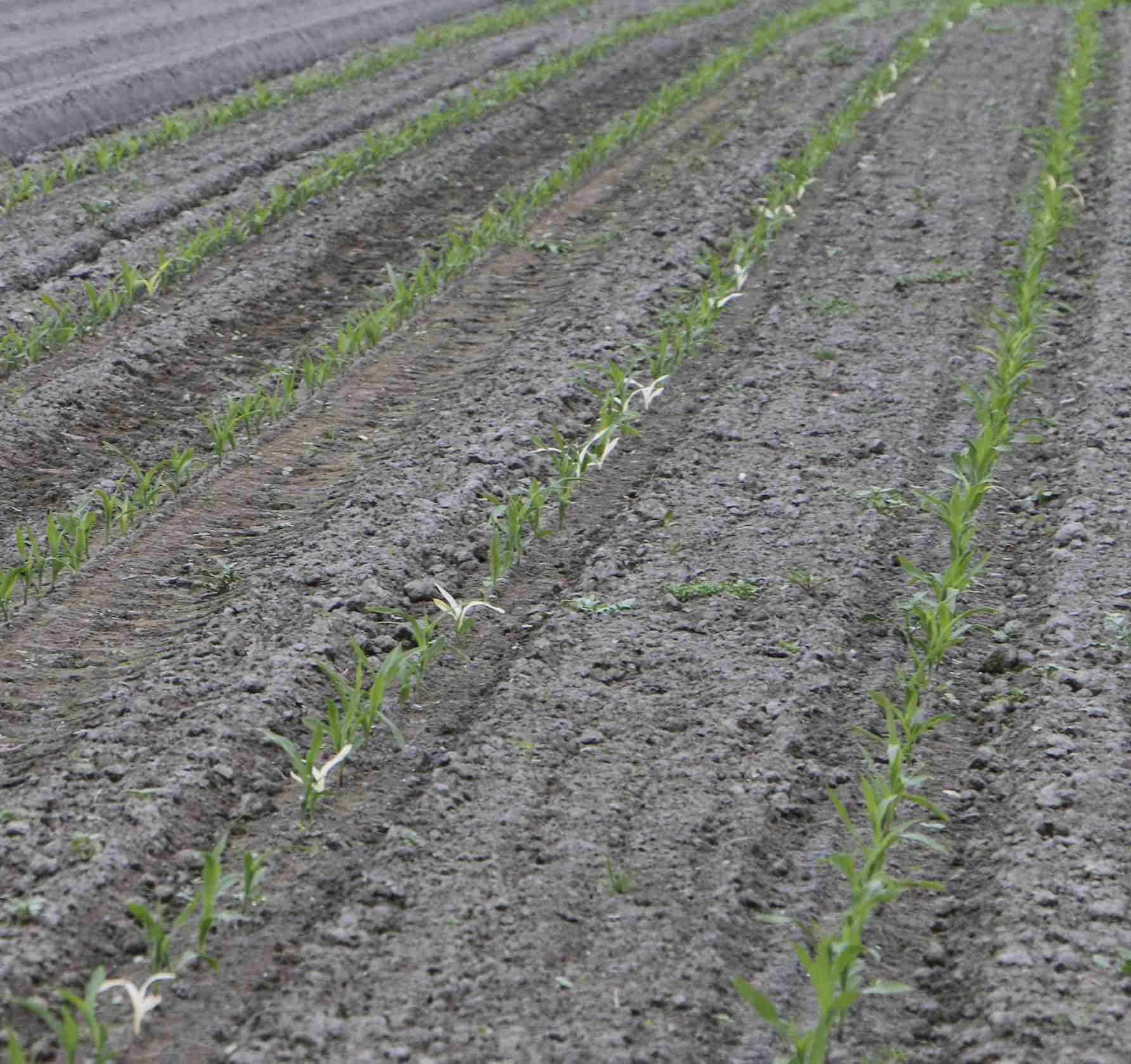
The data set for this exercise consists of 148 genotyped individuals that were prepared in the previous exercise. As a reminder the data span a region of 3 Megabases on chromosome 1 of the maize genome. The individuals belong to teosinte (the wild ancestor of cultivated maize), maize landraces and modern maize varieties. First, load the data set that you saved as an Rdata objects in the first computer lab:
load("data/zea_snps.RData")
load("data/teosinte_acc.Rdata")
load("data/landraces_acc.Rdata")
load("data/varieties_acc.Rdata")
Genetic diversity
We will look at the genetic diversity within each of the three data sets.
The function seg.sites returns the indices (positions) segrating sites in a data frame, which can then be counted using the length() function.
First we calculate the number of variants, i.e. the number of segregating sites \(S\). For a nice presentation of the output, a data frame is constructed and it is converted to a nice-looking table using the knitr::kable() function
# Calculate the number of segregating sites for each pool
teosinte_seg <- length(seg.sites(zea_snps[teosinte_acc,]))
landraces_seg <- length(seg.sites(zea_snps[landraces_acc,]))
varieties_seg <- length(seg.sites(zea_snps[varieties_acc,]))

# Create a data frame with the results
result_table <- data.frame(
  Pool = c("Teosinte", "Landrace", "Variety"),
  `Segregating sites` = c(teosinte_seg, landraces_seg, varieties_seg)
)

# Display the table nicely using knitr::kable()
knitr::kable(result_table, caption = "Segregating Sites by Pool")
Next, we calculate the nucleotide diversity \(\pi\):
n_snps <- ncol(zea_snps) # get the number of SNPs in the 3 MB long region
pi_teosinte <- (nuc.div(zea_snps[teosinte_acc,])*n_snps)/3000000
pi_teosinte
pi_landraces <- (nuc.div(zea_snps[landraces_acc,])*n_snps)/3000000
pi_landraces
pi_varieties <- (nuc.div(zea_snps[varieties_acc,])*n_snps)/3000000
pi_varieties
The reason why we first multiply with the reported number of variants in this data set and then divide by the sequence length is that we want to have a per site estimate and the original vcf input data file did only contain the variant positions.
It is easy to compare the effect of correcting for the length of the sequenced region.
Compare the output of the command nuc.div(zea_snps[teosinte_acc,]) with the output of `pi_teosinte <- (nuc.div(zea_snps[teosinte_acc,])*n_snps)/3000000``
Why is the output of the first command higher than of the second command?
Please review the formula to calculate nucleotide diversity that you learned about in the lecture.
Modify the above code to include the value of pi as another column in the table.
- Which data set has the highest genetic diversity? Which one the lowest?
- Can you come up with an explanation of the differences in genetic diversity?
Sliding window analysis
The above calculation gives an average nucleotide diversity for the whole 3 megabases long region. There is, however, the expectation that there is some variation in genetic diversity within this region. We therefore use a sliding window approach to calculate nucleotide diversity in windows of 10000 bp that slide along the chromosomes in steps of 100 bp.
Before we can start with the sliding window analysis, we have to get the position of each polymorphism. Unfortunately, the DNAbin object does not store the chromosome and position on the chromosome in the object, but it is encoded in the column name of the object because the vcfR package reads the chromosome number and position from the vcf file and then encodes it. Therefore, S1_265004016 reflects the position 1_265004016 on chromosome 1.
We have extract from the column names of the DNAbin object and then extract the position and chromosome.
First, load the stringr library for string manipulation.
# install.packages("stringr") # run only once
library(stringr)
To be able to analyse different populations, we define a large function analyse_sliding_window. The function first creates windows and then iterates over them. Instead of using a for loop for the iteration, which is slow in R, we use the sapply function to serially apply a function to the data.
window_size <- 10000       # Window size: 10,000 base pairs
step_size <- 10000           # Step size: 100 base pairs
analyse_sliding_windows <- function(snp_data, window_size, step_size) {
# Get the polymorphism names from the DNAbin object
polymorphisms <- colnames(snp_data)
# Use regex to extract the chromosome and position components from each name.
# The regex "^S(\\d+)_(\\d+)$" captures two groups: chromosome (group 1) and position (group 2)
matches <- str_match(polymorphisms, "^S(\\d+)_(\\d+)$")
# Convert the captured values to numeric
chromosome <- as.numeric(matches[, 2])
position <- as.numeric(matches[, 3])
# Get starting and end positions on the chromosome.
# Here we assume the positions are sorted in ascending order.
startpos <- position[1]
endpos <- tail(position, 1)
# Generate the starting positions for the sliding windows
starts <- seq(startpos, endpos - window_size + 1, by = step_size)
# Calculate the midpoint for each window (used as the position indicator)
midpoints <- starts + floor(window_size / 2)
# Calculate nucleotide diversity per nucleotide for each window.
# Here we divide the nucleotide diversity (calculated by nuc.div on the window) by the window size.
nuc_diversity <- sapply(starts, function(start) {
# Define the end position of the window
end <- start + window_size - 1
# Subset polymorphisms based on chromosome 1 and the current window
selected_polymorphisms <- polymorphisms[chromosome == 1 & position >= start & position <= end]
# Extract the corresponding columns from the DNAbin object
selected_snps <- snp_data[, selected_polymorphisms, drop = FALSE]
# Calculate nucleotide diversity over the window (using nuc.div from the pegas package)
diversity <- nuc.div(selected_snps)
# Return the nucleotide diversity per nucleotide
diversity / window_size
})
# Combine midpoints and nucleotide diversity values into a data frame
results_df <- data.frame(
Midpoint = midpoints,
Nucleotide_Diversity = nuc_diversity
)
return(results_df)
}Run the function for the complete dataset and then plot the diversity along the chromosome.
zea_snps.div <- analyse_sliding_windows(zea_snps, window_size, step_size)
teosinte_snps.div <- analyse_sliding_windows(zea_snps[teosinte_acc,], window_size, step_size)
landraces_snps.div <- analyse_sliding_windows(zea_snps[landraces_acc,], window_size, step_size)
Now plot the level of diversity along the chromosome. We use ggplot2 for the plotting, and for this purpose, we create a dataframe with the diversity values. Since the midpoints are the same for all, we can easily combine them into a new dataframe for the plotting
df_plot <- data.frame(
  Midpoint = zea_snps.div$Midpoint,
  Zea_Div = zea_snps.div$Nucleotide_Diversity,
  Teosinte_Div = teosinte_snps.div$Nucleotide_Diversity,
  Landraces_Div = landraces_snps.div$Nucleotide_Diversity
)
Then plot the dataframe
library(ggplot2)ggplot(df_plot, aes(x = Midpoint)) +
#geom_line(aes(y = Zea_Div, color = "Zea Diversity"), size = 1) +
geom_line(aes(y = Teosinte_Div, color = "Teosinte Diversity"), size = 1) +
geom_line(aes(y = Landraces_Div, color = "Landraces Diversity"), size = 1) +
labs(x = "Midpoint", y = "Nucleotide Diversity", color = "Group") +
theme_minimal()- Add the code for the
varietiesto plot the variation along the chromosome. - Which general patterns do you recognize with respect to the overall levels of diversity and the variation in genetic diversity along the chromosome in the different pools of the sample?
- Which explanations can you come up with to explain the high variation of diversity levels along the chromosome?
- Can you think of any biases with respect to the total levels of diversity and the levels of diversity in individual genomic regions? (Hint: Think of the effect of the filtering during data preparation or in later stages of the analysis)
Identification of outlier windows
The comparison of diversity levels of individual windows between pools may provide further insights.
We can use a scatterplot and a linear model to identify windows, whose level of diversity differs strongly between pools.
# Calculate the maximum value for the limits (ignoring NA values)
max_val <- max(c(df_plot$Teosinte_Div, df_plot$Landraces_Div), na.rm = TRUE)

ggplot(df_plot, aes(x = Teosinte_Div, y = Landraces_Div)) +
  geom_point() +
  # Add the x = y line (dashed line)
  geom_abline(intercept = 0, slope = 1, linetype = "dashed", color = "gray") +
  # Fit and add the linear model line without confidence interval (blue line)
  geom_smooth(method = "lm", se = TRUE, color = "blue") +
  # Set x and y limits the same based on the maximum value
  scale_x_continuous(limits = c(0, max_val)) +
  scale_y_continuous(limits = c(0, max_val)) +
  labs(
    x = "Teosinte Nucleotide Diversity",
    y = "Landraces Nucleotide Diversity",
    title = "Scatterplot of Nucleotide Diversities: Teosinte vs Landraces",
    subtitle = "Dashed line: x = y | Blue line: Linear Model Fit"
  ) +
theme_minimal()- Make a similar plot for the comparison of Landraces versus Varieties diversity.
- Interprete the resulting plots. What to the lines indicate?
- Which approach would you take to (statistically) identify and further characterize outliner windows?
- Which process could explain the presence of the outlier windows?
Exercises
- Calculate gene diversity for a tri-allelic marker and the following allele frequencies:
| \(p_1\) | \(p_2\) | \(p_3\) | Gene diversity, \(H\) |
|---|---|---|---|
| 0.1 | 0.1 | 0.8 | |
| 0.333 | 0.333 | 0.333 | |
| 0.5 | 0.25 | 0.25 | |
| 0.998 | 0.001 | 0.001 |
For which marker frequencies is \(H\) the highest? Which conclustion can you draw from the \(H\) values?
- Calculate the parameters of the sequence alignment:
seq1 GATCTATATA
seq2 GAACTATATA
seq3 CATCATCATA
seq4 GACCTATATC
Calculate the following parameters \(n\) (sequence number), \(L\) (sequence length), \(S\) (segregating sites), nucleotide polymorphisma, \(P\), and nucleotide diversity, \(\pi\).