Demographic analysis

Motivation

In addition to molecular genetic analyses of domestication, characterizing the demographic history of crop domestication and evolution provides critical insights into how crops originated and diversified, thus improving our ability to utilize plant genetic resources effectively. Taking maize as a concrete example, researchers have shown that domestication occurred around 9,000 years ago in southern Mexico, where wild teosinte plants were selectively bred by early farmers. Understanding precisely when and where domestication took place helps us reconstruct historical patterns of population structure and migration events that shaped modern maize diversity. Moreover, examining how much genetic variation was lost during maize domestication reveals the severity of the genetic bottleneck that occurred, which is useful information for developing strategies for genetic conservation and improvement. Identifying specific genes and phenotypes that carry footprints of selection further elucidates the evolutionary forces imposed by human cultivation and breeding practices. Therefore, we specifically explore methods designed to detect selected genes, as these techniques complement traditional genetic analyses (i.e., QTL mapping) by highlighting genes crucial for crop adaptation and ongoing breeding programs.

Learning goals

1. Understand the principles of detecting artificial selection in crop genomes using population genetic methods.
2. Identify and differentiate between adaptive, domestication, improvement, and neutral genes in the context of crop evolution.
3. Apply concepts such as mutation-drift equilibrium and selective sweeps to interpret patterns of genetic variation in domesticated plants.

Population genetics of crop domestication: Detection of anthropogenic selection

It can be expected that genes which control the domestication syndrome evolved under strong artificial selection because plants with useful mutations were selected by early farmers. There should be significant differences in frequencies of alleles at these genes between wild ancestors and domesticated varieties.

Such genes can be identified by searching for genes with a ‘footprint’ of selection by comparing patterns of genetic variation within and between species (or between wild ancestors and crops derived from them). Genomic regions with unusual patterns of polymorphisms are identified. Such an approach pinpoints domestication genes that were indirectly selected and may be missed in QTL studies because of a subtle effect on the phenotype that is difficult to detect in phenotypic analyses.

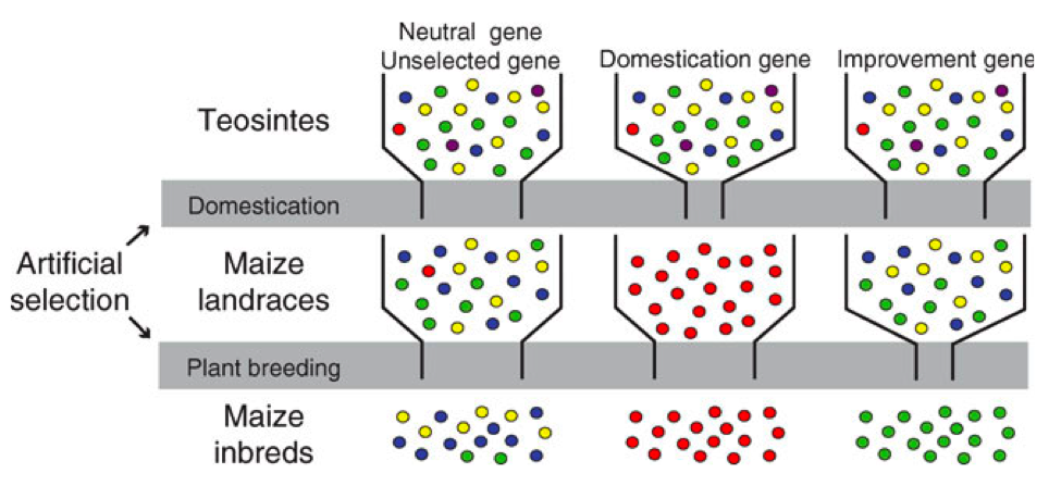
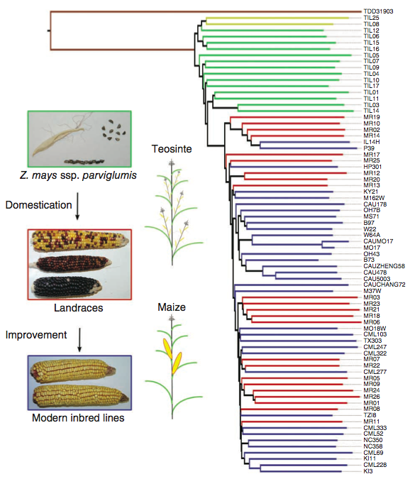
As we already discussed, different types of genes are expected to have experienced selection at different stages of the evolution of crops (Figure 1)

Adaptive trait genes

These genes contain alleles that in natural populations respond to natural selection on environmental conditions because they control adaptive traits. They are good candidates for a transfer into elite germplasm (e.g., drought resistance genes, disease resistance genes). They are expected to be less polymorphic in landraces and modern varieties than in wild ancestors because genetic drift during the domestication bottleneck and modern plant breeding reduced their diversity.

Domestication genes

These genes harbor alleles that were fixed during domestication. They were exposed to strong selection during domestication and are expected to be essentially monomorphic (i.e. lack polymorphism) in both land races and modern varieties, but not in wild ancestors.

Yield improvement

These genes are the target of artificial selection in modern breeding programmes. They were not exposed to selection in the wild ancestor and during domestication, but they are exposed to selection in modern breeding programs.

Neutral genes

Such genes were not selected in wild ancestors, during domestication and during plant breeding. Most likely, this is the largest class of genes and they have important functions for the function of the organism. They evolve under purifying selection, but are not the target of positive selection. Changes in genetic diversity during domestication and plant breeding result from genetic drift or linkage with selected genes.

Figure 1: Selection at different types of genes at different stages of crop evolution. Source: Yamasaki et al. (2005)

Methods for detecting selection

Several general approaches are possible for using sequence data to search for signs of selection. They all have in common that they are used to test whether the null hypothesis of ** a model of neutral evolution** can be rejected.

Tests that are based on pattern of within-species polymorphism can be used to detect ongoing or recent selection (Tajima’s \(D\) would be such a test¹. An example is the analysis of genetic variation in maize landraces and and modern, improved varieties.

¹ See chapter on tests of neutral evolution: Link

Tests that are based on polymorphism plus between species divergence that also detect ongoing or recent selection. They are based on the notion that without selection, the rate of evolution of genes between and the genetic diversity withing should be correlated because they are influenced by the same neutral processes: Mutation and drift. An example would be the comparison of the genetic diversity of maize and its wild ancestor teosinte, or the wild relative Tripsacum dactyloides.

Tests that are based on phylogenetic comparisons between species. They are most suited for detecting historical selection, selection far back in time. An example is the comparison of maize, teosinte, rice, sorghum, wheat and barley using phylogenetic methods.

The mutation-drift equilibrium

To introduce the analysis of selection in the context of selection, we recapitulate the population genetic basis of selection detection.

Mutation creates new genetic variation and genetic drift removes it. Even though alleles change over time, the heterozygosity of a population remains largely constant in an equilibrium, which is called mutation-drift equilibrium². If a population has reached a mutation-drift equilibrium, the expected level of polymorphism at a gene within a population is the product of the effective population size, \(N_e\) and the mutation rate, \(\mu\), \[\begin{equation} \label{mutdrift} H = 4N_e\mu. \end{equation}\] The mutation-drift equilibrium is also the basis of the Neutral Theory of Molecular Evolution, which was mainly developed by the Japanese geneticist Motoo Kimura and has been of great importance in molecular evolution and population genetics because this theory makes very simple and testable predictions about the expected levels and patterns of polymorphisms in populations Kern and Hahn (2018).

² For a derivation of the following theory, you may want to check any introductory textbook on population genetics

Mutation and drift also generate a between-line variance, i.e., a population divergence. As lines separate, the initial heterozygosity is randomly partitioned, creating between-line variance. More importantly, as new mutations arise in the separated lines, some of these are fixed by drift, and this drives a constant divergence between populations.

Figure 2: Genetic divergence of populations by genetic drift without selection. Source: Unknown

One average, for a population of size \(N\), \(2N\mu\) mutations arise each generation. For any of these, their probability of fixation is \[P_{\text{fixation}} = 1/(2N) \tag{1}\] Hence, the rate at which new mutations are fixed within a line is just the number of new mutations per generation and the chance of their fixation: \[2N\mu\times1/(2N) = \mu \tag{2}\] The divergence \(d(t)\) after \(t\) generations is then \[d(t) = \mu t. \tag{3}\] Note that the divergence is independent of the population size! The neutral theory makes several predictions that can be used for tests of selection:

• Within population variation: \(4N_e\mu\)
• Rate of divergence per generation: \(\mu\)
• Between population variation: \(2t\mu\)

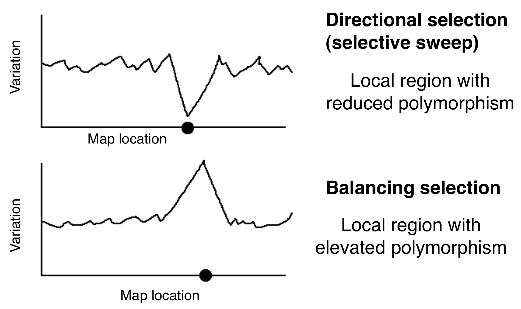
These results can be used to design a test that is based on the analysis of polymorphisms. The goal is to compare the time of observed MRCA to the time expected under a neutral mutation-drift model. If a locus evolved under positive selection, the MRCA should be more recent. In other words, the coalescent is shorter. If a locus evolves under balancing selection, the MRCA should be older relative to drift and the coalescent should be deeper. A shorter coalescent translates into a locus with lower levels of variation and longer blocks of disequilibrium. A deeper coalescent is associated with higher levels of variation and shorter blocks of disequilibrium (Figure 3).

Figure 3: Relationship between the type of selection and the coalescent. Source: Walsh (2008)

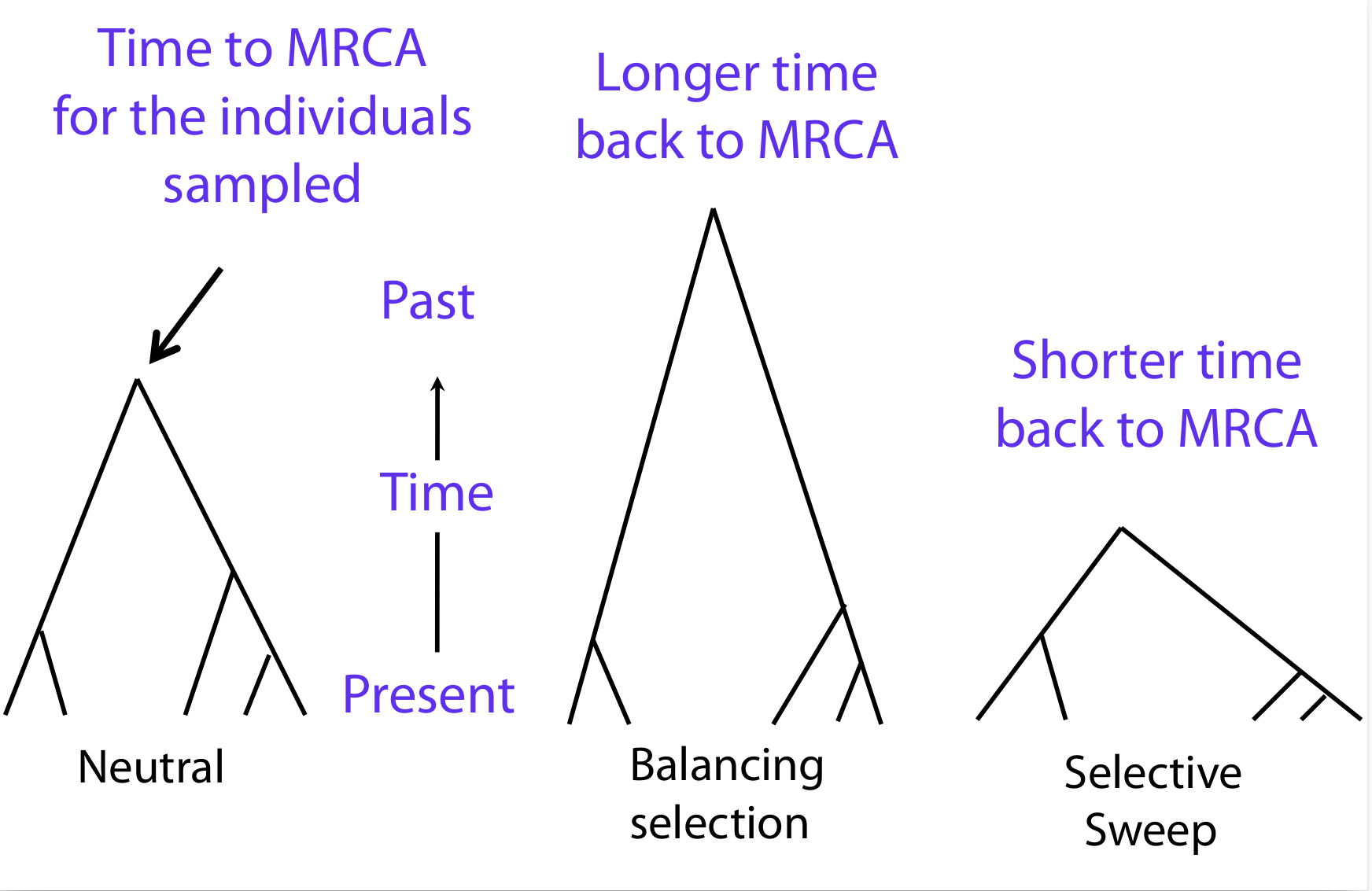
Selective sweeps result in a local decrease in \(N_e\) around the selected site, which results in a shorter time to MRCA and a decrease in the amount of polymorphisms. This has no effect on the rate of divergence of neutral sites between populations, as this is independent on \(N_e\). Conversely, balancing selection increases the effective population size, which increases the amount of polymorphism.

Figure 4: Detection of selection by scans of levels of polymorphism in the genome. Source: Walsh (2008)

To summarize, coalescent theory provides a framework to analyse the extent of polymorphism at a locus and to produce null hypotheses of genetic variation under a neutral model that can be used to test for selection.

Selection at the teosinte-branched 1 gene

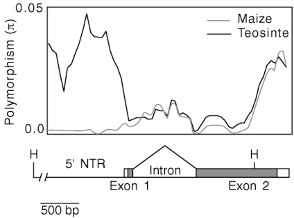
The theory introduced in the previous section was applied to study selection of a domestication gene in maize. John Doebley and co-workers reasoned that because of its effects on the genetic architecture of maize, the teosinte-branched 1 gene should show a footprint of selection associated with domestication. They sequenced the gene both in maize and teosinte accessions and observed a significant decrease in genetic variation in the 5’ NTR (non-translated region) of tb1, which suggested that a selective sweep influenced this region. In contrast, the coding region of the gene was not influenced by this sweep.

Figure 5: Comparison of nucleotide diversity at the tb1 locus in teosinte and maize. While the genetic diversity in the protein is similar between both teosinte and maize, diversity is strongly reduced in the upstream region. Wang et al. (1999)

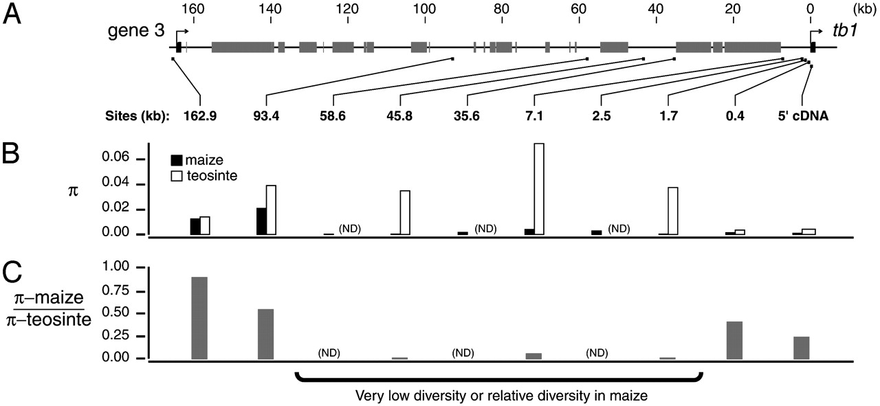
To further characterize genetic diversity between maize and teosinte, the region between the next gene (gene3) located upstream of tb1 was sequenced in both teosinte and maize genotypes. The results indicated a strong reduction of diversity up to 46 kilobases upstream of the tb1 protein coding region, consistent with a strong selective sweep in the region (Figure 6). This pattern is consistent with a strong local selective sweep as shown in Figure 4.

Figure 6: (A) The location of sampled sites relative to sequence features in the gene 3 to tb1 region. (B) The levels of nucleotide diversity (\(\pi\)) for maize and teosinte. (C) The relative ratio of \(\pi\) n maize to teosinte. Values of \(\pi\) for teosinte were calculated from combined subsp. parviglumis and subsp. mexicana sequences. ND, regions for which teosinte data are not determined. Source: Clark et al. (2004)

Both studies used the wild ancestor teosinte as a control to estimate the extent of a genome-wide reduction of neutral polymorphisms in maize caused by the domestication bottleneck.

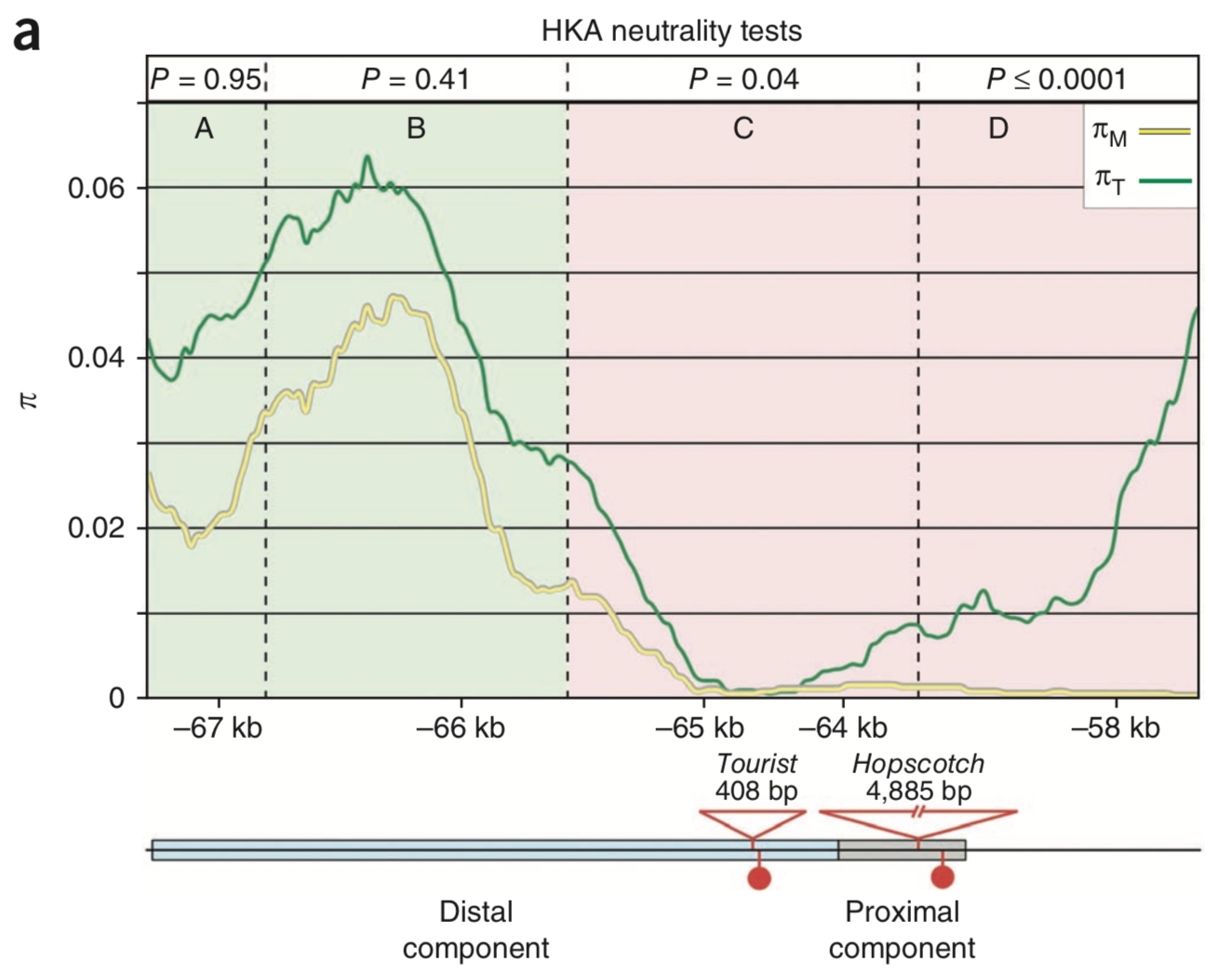
Genetic studies identified the insertion of a transposable element (TE9 of the Hopscotch TE family in a control region (CR) about 64 kilobases upstream of the tb1 start codon as causal mutation for the domestication phenotype. This finding was confirmed by a test of selection of the region harboring this Hopscotch insertion. Studer et al. (2011) conducted an Hudson-Kreitman-Aguade (HKA) test, which compares intraspecific diversity with interspecific divergence (Figure 7). According to the neutral theory of molecular evolution, the ratio of intraspecific diversity between divergence and polymorphisms for different taxa should be the same if a locus evolves neutrally without any selection. In the control region of tb1 the test was highly significant in the region of the proximal component of the CR, indicating a local selective sweep.

Figure 7: Sequence diversity in maize and teosinte across the control region. (a) Nucleotide diversity across the tb1 upstream control region (CR). Base-pair positions are relative to AGPv2 position 265,745,977 of the maize reference genome sequence. P-values correspond to HKA neutrality tests for regions A–D, as defined by the dotted lines. Green shading signifies evidence of neutrality, and pink shading signifies regions of non-neutral evolution. Nucleotide diversity (\(\pi\)) for maize (yellow line) and teosinte (green line) were calculated using a 500 bp sliding window with a 25-bp step. Source: Studer et al. (2011)

Taken together, the analysis of genetic diversity in the upstream region of tb1 provided strong evidence that genetic diversity was reduced due to selection of the domestication allele in maize. The ancient DNA study presented earlier supports this evidence.

Estimating the strength of selection

The strength of a selective sweep can be estimated from the size of the sweep region. The distance \(d\) at which a neutral site can be influenced by a sweep is a function of the strength of selection, \(s\), and the recombination fraction, \(c\), with \(d \approx 0.01\times s/c\) (Kaplan et al., 1989). Hence, \(s = 100 \times d \times c\). For \(tb1\), \(s\) was estimated as 0.05. With \(s\) in hand, one can also estimate the expected time for selection to fix the allele, which was estimated at 300 to 1,000 years, indicating a fairly long period of domestication (Wang et al., 1999).

Selection in the waxy gene of rice

A similar pattern of the effect of strong artificial selection can be seen in the Waxy gene (Olsen et al., 2006). ‘Sticky’ (glutinous) rice grains results from low amylose levels, and are typical of temperate japonica variety groups. Several research groups showed this is due to a gene-splicing mutant in the Waxy gene. This is an example of an improvement gene (as opposed to a domestication gene). The authors observed a region 250 kb in size around Waxy with a greatly reduced level of polymorphism compared to control populations.

Figure 8: Ratio of genetic diversity between two groups of rice genotypes defined whether they carry the wild type or the splicing mutant. Diversity is also reduced in neigbhoring genes. Source: Olsen et al. (2006)

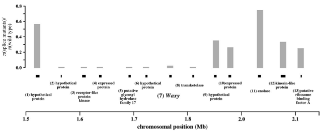
Using the expression from Kaplan et al. (1989), they obtained \(s= 4.6\). While the sweep around \(tb1\) did not even influence the coding region of that gene, the Waxy sweep covers 39 rice genes, indicating that a much larger region of the rice genome was affected by the sweep.

Genome-wide analysis of selection during domestication and improvement

To estimate the extent of selection during domestication in the whole genome, and to compare the patterns of selection during post-domestication plant improvement (i.e., modern scientific breeding), the genomes of 75 maize lines was resequenced (Hufford et al., 2012).

Figure 9: Geographic origin of landraces included in the survey of genome-wide diversity. Source: Hufford et al. (2012)

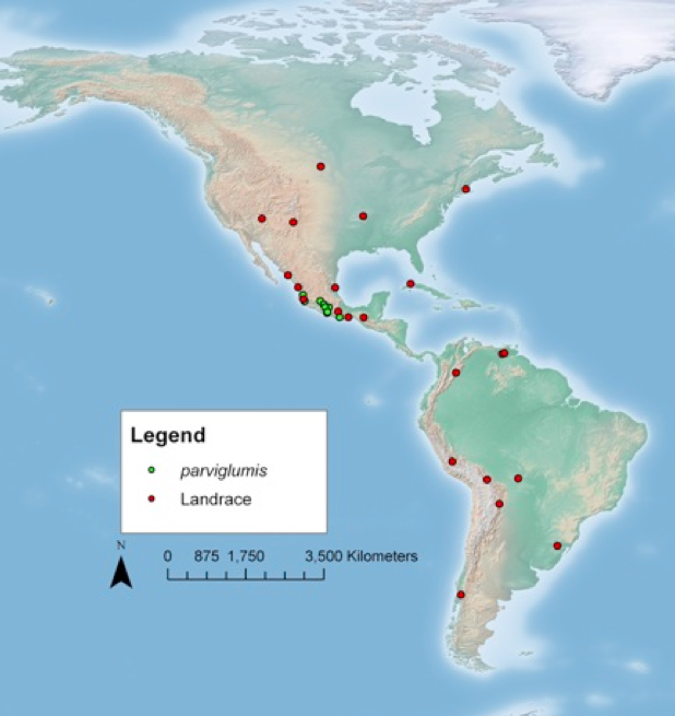
This set included:

• 35 improved maize lines
• 21 traditional landraces from Latin America
• 14 teosinte Zea mays ssp. parviglumis)
• 2 teosinte Zea mays ssp. mexicana
• 1 relative species Tripsacum dactyloides var meridionale

The geographic origin of the landraces included in the study is shown in Figure 9. The sequencing of the 75 lines resulted in 21 Million SNPs. A phylogenetic analysis of the SNPs indicated a clear separation of teosinte from the cultivated maize lines, but not a separation of landraces and improved lines (Figure 10).

Figure 10: Neighbor-Joining tree of the lines sequenced in the domestication study. Taxa in the neighbor-joining tree (right) are represented by different colors: parviglumis (green), landraces (red), improved lines (blue), mexicana (yellow) and Tripsacum (brown). Source: Hufford et al. (2012).

Table 1: Different diversity statistics in the three sequenced groups. \(\rho\) is the population recombination parameter (\(\rho = 4N_{e}r\), with \(r\) as recombination rate). Source: Hufford et al. (2012)

Statistic	parviglumis	landrace	improved
\(\pi\)	0.0059	0.0049	0.0048
\(\pi_{genic}\)	0.0083	0.0072	0.0071
Tajima’s \(D\) 0	.0412 -	0.0716 -	0.2132
Tajima’s \(D_{\text{genic}}\) 0	.4475 0	.4543 0	.4129
\(\rho\)	0.0088	0.0022	0.0016
\(\rho_{\text{genic}}\)	0.0139	0.0040	0.0024

Compared to the teosintes, 83% of the genetic diversity was retained in the cultivated varieties (Table 1). This is much less of a reduction than was observed in other crops and was explained with the high population size of cultivated maize as well as with the outcrossing habit of maize.

However, in the landraces, there is a high level of linkage disequilibrium. The recombination population parameter, \(\rho = 4N_er\), where \(r\) is the recombination rate per generation, is only 25% of teosinte. In other words, only a quarter of the recombination events is observed in the maize landraces than in the teosintes.

On a genome-wide level, there is an excess of rare alleles suggesting that the population experienced a domestication-associated bottleneck and rapid subsequent population growth (see the chapter on coalescent theory). However this signal is much weaker in coding regions, probably because background selection (purifying selection that removes deleterious polymorphism) is stronger in genic regions.

Although parviglumis teosinte is the direct ancestor of maize, the sequence analysis also showed strong evidence for the introgression of alleles from mexicana subspecies of teosinte into maize.

Detection of selected regions in the maize genome

Genomic regions and genes which were selected during domestication or plant improvement by comparing significant differences in gene frequencies of genomic regions between teosinte and landraces to detect domestication genes, as well as between landraces and improved varieties to identify plant improvement genes. Regions that contained a significant number of such differences were called ‘features’.

Figure 11 shows the diversity of teosinte and maize in chromosome 1, as well as tests of selection for domestication and improvement genes. The XP-CLR test is a test of selection that measures genetic differentiation between two groups caused by selection. The effect of domestication-related selection were identified by applying the test to teosinte versus all landraces, and the effect of domestication-related selection was identified by applying the test to landraces versus improved linnes.

Figure 11: Genome-wide analysis of nucleotide diversity and selection. (a) Lowess curves of nucleotide diversity (\(\pi\)) along chromosome 1 in parviglumis (green), landraces (red) and improved lines (blue). (b,c) Genome-wide likelihood (XP-CLR) values for selection during domestication (b) and improvement (c) Source: Hufford et al. (2012)

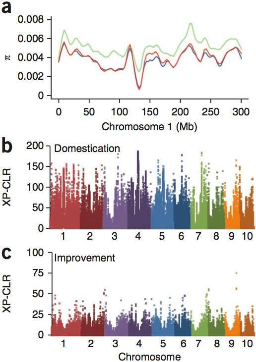
Of the top 10% of each class were 484 domestication and 695 improvement features (i.e., genomic regions with a signature of selection). Domestication features contained an average of 3.4 genes, had a mean size of 322 kb covered approximately 7.6% of the maize genome (Figure 12).

Figure 12: Distributions of feature size (a) and gene counts within features (b) in domestication and improvement scans. Whiskers indicate maximum and minimum of data, boxes span the interquartile range, and the solid line indicates the median. Source: Hufford et al. (2012)

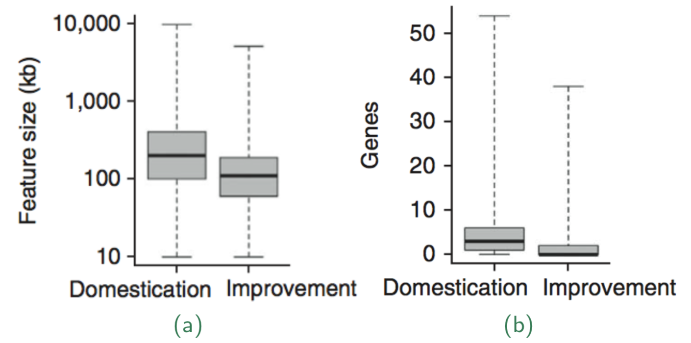
The average selection coefficients, estimating the strength of selection are given in Table Table 2. Because of the weaker selection, the improvement feature were smaller and contained fewer genes.

Table 2: Average selection coefficients estimated for domestication and improvement features identified in tests of selection. Source: Hufford et al. (2012)

Feature	Selection coefficient (\(s\))
Genome-wide	0.0011
Domestication	0.015
Improvement	0.003

About 26% of the domestication and the improvement features were overlapping, which suggests that plant breeding at least partially affects the same genes as in domestication. This suggest that domestication genes still contribute to agronomic performance in current plant breeding programs. In addition to a change in allele frequencies the domestication genes also showed a stronger change in expression level than improvement candidate genes and randomly chosen genes. This indicates that changes in the patterns of gene expression are an important aspect of genome evolution.

A comparison of the newly detected domestication features (i.e., genes) compared to known candidate genes such as teosinte-branched 1 (tb1) shows that they have stronger selection coefficients and are assigned to different biological functions. This strongly indicates that in addition to the morphology-altering mutations, many other as yet unknown processes played a role in domestication.

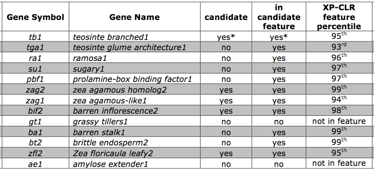
The tests of selection can also be used to test whether the known and novel domestication genes are included among the identified features. Table 3 shows that most of the known domestication genes, including tb1 were identified in this screen, in addition to many novel genes whose genetic diversity was changed due to selection in domestication or subsequent improvement.

Table 3: Table with genes whose genetic diversity was significantly changed during domestication or improvement by selection. Source: Hufford et al. (2012)

Demographic history of plant genetic resources

We can apply the theory further to study the population history of crop species or their wild relatives.

Figure 13: Model of the demographic history of wheat. \(N_A\),\(N_L\),\(N_C\): pop. sizes of ancestral, landrace, and cultivar populations. \(T_1,T_2\): start, stop of bottleneck. Source: Cavanagh et al. (2013)

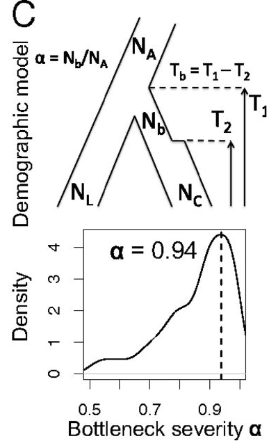
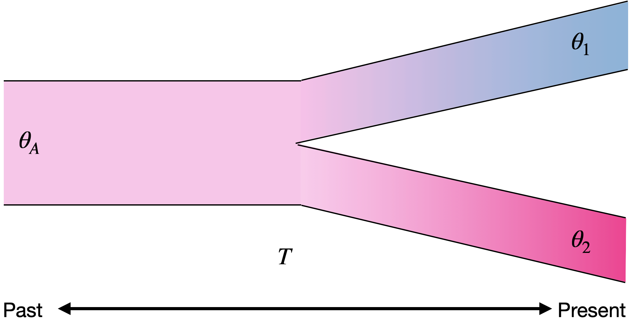
Such a model can be used as a tree model for closely related OTUs in model-based phylogenetics (e.g. with the BEAST approach, Bouckaert et al. (2014)). The approach is to reconstruct the domestication history, estimate times of bottlenecks (periods of reduced \(N\) resp. \(N_e\)) And then find specific genomics regions under selection by taking the demographic history, which affects the whole genome in a similar fashion, under account.

In the context of plant genetic resources, there are many potential applications for this approach. Think about the history of Brassica oleracea vegetables. Diversification of these crops happend fairly recently. After modeling the demographic history of the different types of this vegetable (Broccoli, cauliflower, etc.), one may apply selection tests to identify genomic regions that were selected by humans in the recent history of this crop.

Key concepts

• Demographic history of the whole genome vs. gene specific evolution
• Adaptive trait
  
• Neutral theory of molecular evolution
• [ ] Domestication gene

Summary

• Whole genome resequencing reveals novel candidate genes for domestication.
• Genes that play a role in domestication or plant improvement can be identified by genetic mapping, or by selection scans.
• In maize a comparison of genetic mapping methods and selection scans shows that both methods identified several known, but also novel putative domestication genes.
• The molecular and genetic function of candidate domestication genes identified by the analysis of selection signatures need to be further determined

Further Reading

• Charles Darwin, On the Origin of Species, First Chapter. Download at http://www.gutenberg.org/ebooks/2009
• Doebley et al. (2006) - Review of the molecular genetics of crop domestication
• Hartl and Clark, Principles of Populations Genetics, 4th edition, Chapters 7.1 - 7.4.
• Murphy, People Plants and Genes, Chapters 5 and 6.

Study questions

1. What types of genes are expected to show footprints of artificial selection during crop domestication?
2. Explain briefly the mutation-drift equilibrium and how it is used in population genetics to detect selection.
3. What is the difference between a domestication gene and an improvement gene? Give an example of each.
4. Describe one test used to detect ongoing or recent selection within species.
5. What evidence suggests a selective sweep occurred at the teosinte-branched 1 (tb1) locus during maize domestication?
6. How can the strength of selection (selection coefficient, \(s\)) be estimated from genomic data?
7. Explain why selection in the waxy gene of rice resulted in a larger genomic region being affected compared to selection at the tb1 locus in maize.
8. What did genome-wide analyses reveal about genetic diversity retention in maize compared to teosinte?
9. What is linkage disequilibrium, and how did it differ between maize landraces and their wild ancestor teosinte?
10. What is the significance of identifying overlapping genomic regions affected by domestication and improvement selection?

Problems

1. In a very short commentary, Doebley (2006) describes some findings on domestication genetics in other crops. What are his key conclusions with respect to general patterns of crop domestication?
2. Which approaches for the identification of domestication genes are presented by Doebley et al. (2006). Which approach was most successful in their time?

References

Bouckaert R, Heled J, Kühnert D, Vaughan T, Wu C-H, Xie D, Suchard MA, Rambaut A, Drummond AJ. 2014. BEAST 2: A Software Platform for Bayesian Evolutionary Analysis. PLoS Comput Biol 10:e1003537. doi:10.1371/journal.pcbi.1003537

Cavanagh CR, Chao S, Wang S, Huang BE, Stephen S, Kiani S, Forrest K, Saintenac C, Brown-Guedira GL, Akhunova A, See D, Bai G, Pumphrey M, Tomar L, Wong D, Kong S, Reynolds M, Silva ML da, Bockelman H, Talbert L, Anderson JA, Dreisigacker S, Baenziger S, Carter A, Korzun V, Morrell PL, Dubcovsky J, Morell MK, Sorrells ME, Hayden MJ, Akhunov E. 2013. Genome-wide comparative diversity uncovers multiple targets of selection for improvement in hexaploid wheat landraces and cultivars. Proceedings of the National Academy of Sciences 110:8057–8062. doi:10.1073/pnas.1217133110

Clark RM, Linton E, Messing J, Doebley JF. 2004. Pattern of diversity in the genomic region near the maize domestication gene tb1. Proceedings of the National Academy of Sciences 101:700–707. doi:10.1073/pnas.2237049100

Doebley J. 2006. Unfallen Grains: How Ancient Farmers Turned Weeds into Crops. Science 312:1318–1319. doi:10.1126/science.1128836

Doebley JF, Gaut BS, Smith BD. 2006. The Molecular Genetics of Crop Domestication. Cell 127:1309–1321. doi:10.1016/j.cell.2006.12.006

Hufford MB, Xu X, Van Heerwaarden J, Pyhäjärvi T, Chia J-M, Cartwright RA, Elshire RJ, Glaubitz JC, Guill KE, Kaeppler SM, others. 2012. Comparative population genomics of maize domestication and improvement. Nature Genetics 44:808–811.

Kaplan NL, Hudson RR, Langley CH. 1989. The "hitchhiking effect" revisited. Genetics 123:887–899.

Kern AD, Hahn MW. 2018. The Neutral Theory in Light of Natural Selection. Molecular Biology and Evolution 35:1366–1371. doi:10.1093/molbev/msy092

Nei M, Suzuki Y, Nozawa M. 2010. The Neutral Theory of Molecular Evolution in the Genomic Era. Annual Review of Genomics and Human Genetics 11:265–289. doi:10.1146/annurev-genom-082908-150129

Olsen KM, Caicedo AL, Polato N, McClung A, McCouch S, Purugganan MD. 2006. Selection under domestication: Evidence for a sweep in the rice waxy genomic region. Genetics 173:975–83. doi:10.1534/genetics.106.056473

Studer A, Zhao Q, Ross-Ibarra J, Doebley J. 2011. Identification of a functional transposon insertion in the maize domestication gene tb1. Nature Genetics 43:1160–1163. doi:10.1038/ng.942

Walsh B. 2008. Using molecular markers for detecting domestication, improvement, and adaptation genes. Euphytica 161:1–17. doi:10.1007/s10681-007-9465-8

Wang R-L, Stec A, Hey J, Lukens L, Doebley J. 1999. The limits of selection during maize domestication. Nature 398:236–239. doi:10.1038/18435

Yamasaki M, Tenaillon MI, Vroh Bi I, Schroeder SG, Sanchez-Villeda H, Doebley JF, Gaut BS, McMullen MD. 2005. A Large-Scale Screen for Artificial Selection in Maize Identifies Candidate Agronomic Loci for Domestication and Crop Improvement. The Plant Cell 17:2859–2872. doi:10.1105/tpc.105.037242