Show the code
```{r}
library(phytools)
tree <- "((A:2.0,B:1.0):2.3,(C:0.5,D:0.5):4,(E:3.14,F:2.7):0.5);"
phy <- read.newick(text=tree)
plot(phy)
```Understanding the evolutionary relationships helps to elucidate patterns of crop biodiversity, understand the process of domestication and to identify genetic resources that are suitable and available for the improvement of a particular crop species.
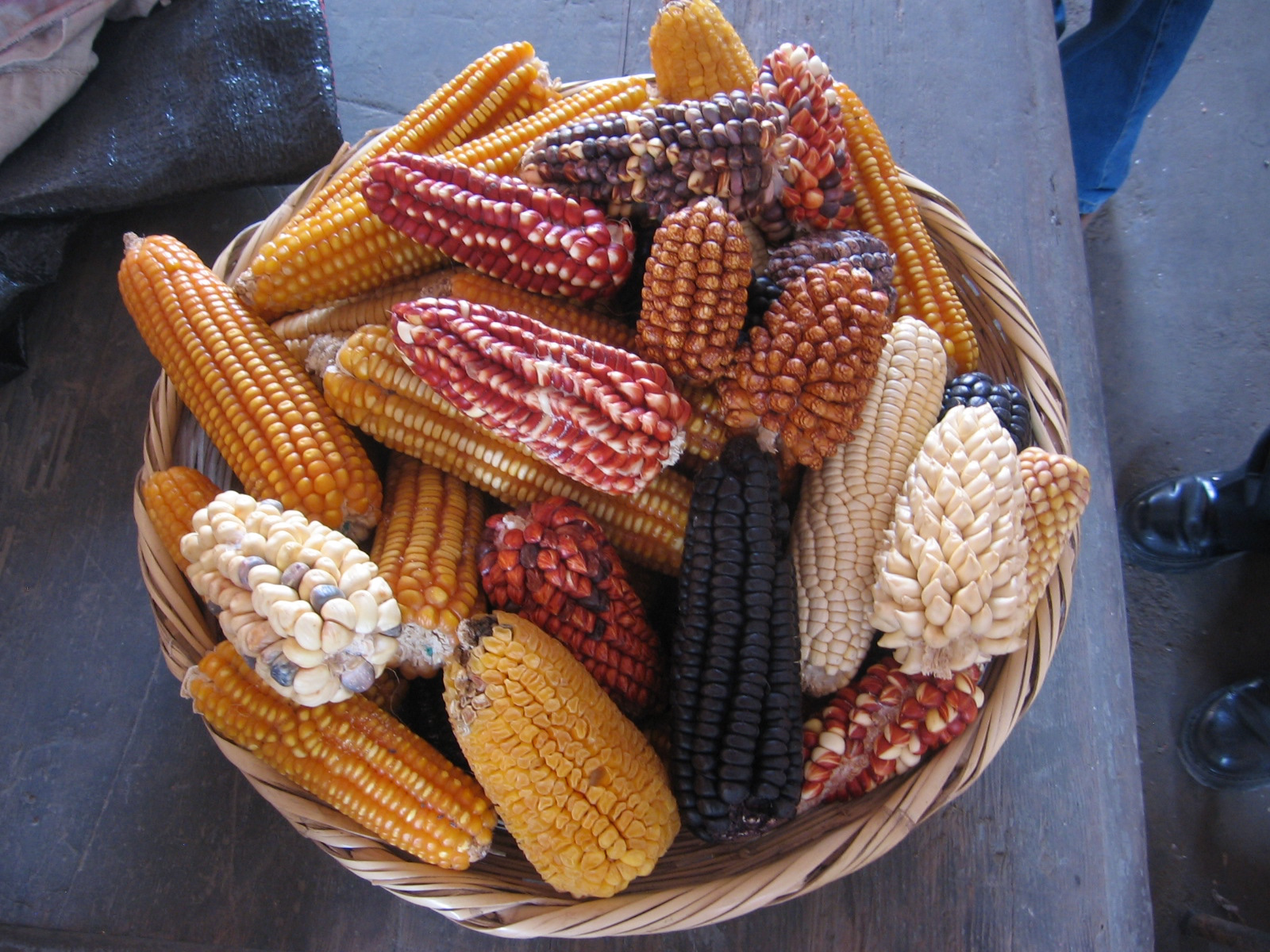
If you recall the diversity of maize landraces in Peru from the introduction (Figure 1) one may ask when and where this diversity originated.
Phenotypic differences between individual plants can be caused by the environment (this variation is not heritable) or by genetic differences, which are heritable. One may safely assume that a large proportion of phenotypic variation that differentiates not individual plants, but landraces or plant varieties is controlled by genetic variation. It is therefore of interest to investigate the extent to which genetic differences are responsible for phenotypic variation in plant genetic resources.
Genetic differences ultimately originate from mutation and recombination. To identify useful genetic variation in plant genetic resources, the following questions are frequent objectives of scientific investigations:
One approach to address these questions is to trace back the evolutionary history of a mutation, a gene, a landrace, or a species using phylogenetics, which we define as the study of evolutionary relationships.
One approach to address these questions is to trace back the evolutionary history of a mutation, a gene, a landrace, or a species.
Methods of phylogenetic analysis or phylogenetic inference, which is the determination of the evolutionary relationship of taxa allow to investigate these questions.
Phylogenetics is an area of evolutionary biology that investigates the evolutionary relationship of species.
Its key metaphor is the evolutionary tree, or phylogeny, that expresses different degrees of evolutionary relationships and states the principle of common ancestry, i.e., that all individuals of a species, or different species of a genus, derive from a common ancestor.
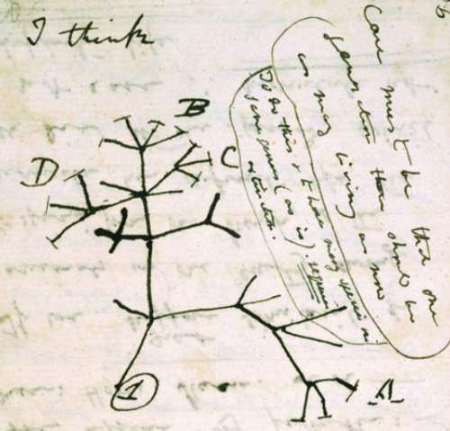
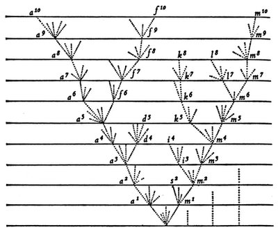
The concept of the evolutionary tree was invented by Charles Darwin who first drew a tree in his notebook (Figure 2) and then put a tree as the only figure in his 1859 book On the Origin of Species (Figure 3). Due to its importance in the analysis of biodiversity, phylogenetics has developed into a mature and highly sophisticated field of biology. Many tools and methods are available for analysing the evolutionary relationship of species but also of individuals within species.
Darwin’s tree already demonstrates three important principles of phylogenetics:
In summary, phylogenetic analysis is a method to group entities that are more similar to each others than to others by reconstructing the ancestral tree. There are numerous questions in the context of plant genetic resources that can be analyzed with phylogenetic methods. They include
A phylogenetic tree consists of nodes and branches (Figure 4). A node connects two branches in strictly bifurcating tree.
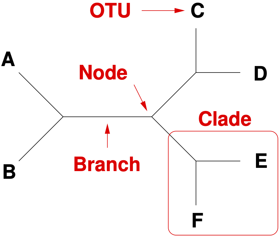
In a multifurcating tree, three or more branches can be connected in a node.
The terminal branches are called leaves, or operational taxonomic units (OTUs). They are the unit of analysis such as species, individuals or genes.
Trees can be rooted or unrooted. In rooted trees, the node with the most recent common ancestor (MRCA) can be identified (Figure 5)
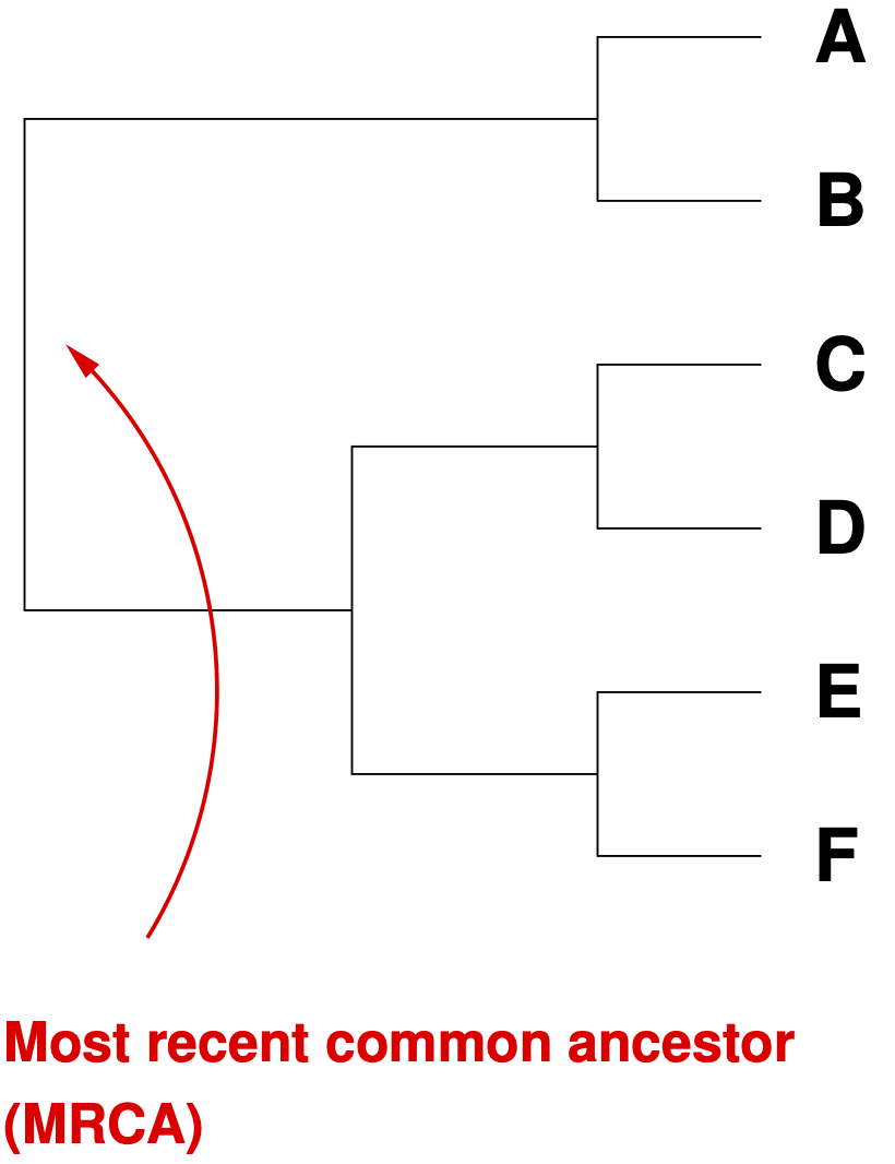
To root a tree, an outgroup OTU is needed. An outgroup is an OTU known (or believed) to be ancestral to all other OTUs in the tree. In crop species, the wild ancestors of cultivated species are often suitable outgroups.
Branches in a tree can be presented scaled or unscaled. If they are scaled, the length of the branches is proportional to the distance of the OTUs that are connected by the branches. The evolutionary distance of OTUs is quantified by a measure. Such measures can be ‘Million years’, or a more abstract measure, such es ‘Mutational distance’ (i.e., the number or proportion of mutations that occurred between two taxa). In coalescence theory, a frequent measure is ‘Number of generations’.
There are two types of common ancestry in a tree. Monophyletic OTUs have a common ancestor in the tree whereas polyphyletic OTUs do not have one.
Phylogenetic trees can be represented as a tree, or in a format that can be read by computers. The most popular computer-readable format is called Newick format. The Newick notation for the tree in Figure 4 is
((A,B),(C,D),(E,F))
The Newick format is also able to express the branch lengths. The same tree as above but with different branch lengths can be expressed as:
((A:2.0,B:1.0):2.3,(C:0.5,D:0.5):4,(E:3.14,F:2.7):0.5)
Phylogenetic trees that were constructed from data such as DNA sequences are inferred trees because it is a tree that was estimated from a particular data set with a certain method. It may or not be the true tree.
Simple code to plot the above tree is shown in the following code1
1 If you want to run this code, you need to install the package phytools first.
```{r}
library(phytools)
tree <- "((A:2.0,B:1.0):2.3,(C:0.5,D:0.5):4,(E:3.14,F:2.7):0.5);"
phy <- read.newick(text=tree)
plot(phy)
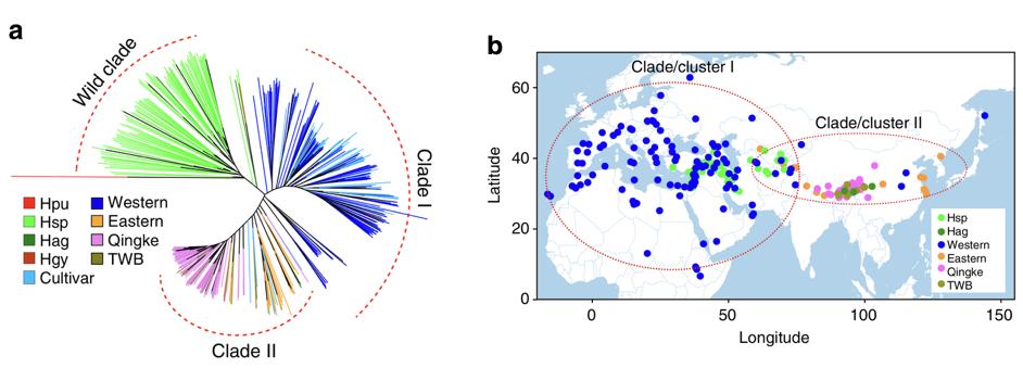
```As a first example of a phylogeny in the context of plant genetic resources, Figure 6 shows the phylogeny of barley landraces (Zeng et al., 2018). It was taken from a study that was aimed at elucidating the evolutionary history of Tibetan barleys, which are morphologically distinct from other barley landraces. The phylogeny shows that Tibetan barleys are also genetically distinct from barley varieties from the region of domestication.
In the following we only consider the construction of phylogenetic trees from SNP markers or DNA sequences. Phylogenies can also be created from other types of data such as phenotypic data.
There are four main methods for constructing phylogenetic trees:
Common to all methods is that they take some form of sequence alignment or data matrix as an input and then calculate a phylogenetic tree.
Distance trees are calculated in two steps. First, a distance matrix is calculated from a multiple sequence alignment. All possible pairwise comparisons of sequences are made and then the pairwise distance is calculated. The result is a \(n\times n\) matrix of pairwise distances. The pairwise distance can be calculated with several methods. In a second step, a tree is calculated from the distance matrix. Frequently used methods are UPGMA (Unweighted Pair Group Method with Arithmetic Mean) or Neighbor Joining (NJ).
If one compares different pairs of sequences, it is obvious that two sequences that differ by 30% of their sequence are less closely related than two sequences that differ by only 10% of their sequences.
Usually, this means that the common ancestor of two divergent sequences is more distant in the past than of two highly similar sequences.
Several methods are available to calculate the distance between a pair of sequences.
They depend on whether the distance is calculated from a matrix of markers (e.g., a 0/1 matrix for a set of markers) or whether DNA or protein sequences are being compared.
SEQ1 GATCTATCTACTACT
SEQ2 ..G.....C....A.
The simplest distance measure is the Hamming distance (Wikipedia), which corresponds to the proportion of nucleotide differences between two sequences. In the above example 3 out of 15 nucleotides differ between the two sequences, and the Hamming distance is therefore 3/15 or 0.2.
Other methods such as Kimura’s distance (Wikipedia) take into account rates of evolution between different nucleotides and are therefore biologically more realistic. For example, it has been observed that usually there is a higher proportion of change from GC to AT nucleotides than vice versa, which can be taken into account into the models. For example the distance accoring two Kimura’s two parameter model is calculated as \[\begin{equation}
K = -\frac{1}{2}\text{ln}((1-2p-q)\sqrt{1-2q}
\end{equation}\] with \(p\) as proportion of sites with transitional differences (purine to purine, \(A \leftrightarrow G\), or pyrimidine to pyrimidine, \(C \leftrightarrow T\) and \(q\) as proportion of sites with transversional differences, (pyrimidine to purine or purine to pyrimidine). In the above example, 1 of 15 sites show a transition and two of 15 sites a transversion, therefore \(p=1/15=0.0666\) and \(q=2/15=0.1333\). The Kimura distance can then be calculated as
```{r}
#| eval: true
K = -0.5*log((1-2*(1/15) - (2/15))*sqrt(1-2*(2/15)))
K
```
[1] 0.2326162UPGMA is the simplest method for clustering. The algorithm finds the pair of taxa with the smallest distance between them and defines the branching point between them als half of that distance. Effectively, a midpoint is placed on the branch. The two taxa are combined into a cluster, which is the substitute for the two taxa. The number of individuals is reduced by one and a new pairwise distance matrix is calculated with all the other sequences. The process is repeated until the matrix consists of a single entry. Then, a tree is reconstructed from the distances.
The following steps are used to construct a UPGMA tree:
The rows and columns of the distance matrix that correspond to \(j\) and \(i\) are deleted and replaced by a row and column of group \(i,j\). If there is only a single cell in the matrix left, the algorithm is finished, otherwise start again. At later stages \(i\) and \(j\) are the newly defined groups and taxa.
The following steps are necessary to calculate a UPGMA tree from the following sequence alignment.
First, get a sequence alignment:
| OTU | 1 | 2 | 3 | 4 | 5 | 6 | 7 | 8 |
|---|---|---|---|---|---|---|---|---|
| A | G | C | A | G | T | A | C | T |
| B | G | T | A | G | T | A | C | T |
| C | A | C | A | A | T | A | C | C |
| D | A | C | A | A | C | A | C | T |
Second, calculate a pairwise distance matrix:
| A | B | C | D | |
|---|---|---|---|---|
| A | 0 | |||
| B | 1 | 0 | ||
| C | 3 | 4 | 0 | |
| D | 3 | 4 | 2 | 0 |
Then select the pair with the lowest distance and calculate a new distance matrix as arithmetic mean with the following equations.
The pair with the lowest distance is \(A, B\). \[\begin{equation} \label{eq-aligned} \begin{aligned} K_{C(A,B)} & = & \frac{1}{2}K_{C,A} + \frac{1}{2}K_{C,B} \\ & = & \frac{1}{2} \times 3 + \frac{1}{2} \times 4 \\ & = & 3.5 \\ \text{Analogous,} \nonumber \\ K_{D(A,B)} & = & \frac{1}{2}K_{D,A} + \frac{1}{2}K_{D,B} \\ & = & \frac{1}{2} \times 3 + \frac{1}{2} \times 4 \\ & = & 3.5 \\ \end{aligned} \end{equation}\] From these calculations, we construct a new table:
| (AB) | C | D | |
| (AB) | 0 | ||
| C | 3.5 | 0 | |
| D | 3.5 | 2 | 0 |
We then select the next pair with the smallest distance, which is C and D, and calculate the new matrix as
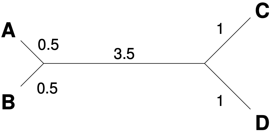
\[\begin{equation} \label{eq-upgmadist} \begin{aligned} K_{(A,B),(C,D)} & = & \frac{1}{2} K_{(A,B),C} + \frac{1}{2} K_{(A,B),D}\\ & = & \frac{1}{2} \times 3.5 + \frac{1}{2} \times 3.5 \\ & = & 3.5 \\ \end{aligned} \end{equation}\]
The new matrix is then
| (AB) | (CD) | |
| (AB) | 0 | |
| (CD) | 3.5 | 0 |
The resulting unrooted tree is shown in Figure 7.
The Neighbor-joining (NJ) method (Wikipedia) is similar to UPGMA because it utilizes a pairwise matrix and reduces the size at each step. However, it calculates distances to internal (rather than external) nodes.
NJ is more frequently used than UPGMA because it does not assume that all taxa are equidistant from a root, which is a biologically very unrealistic assumption.
The maximum parsimony (MP) method attempts to find a tree that is constructed with the least number of substitutions to explain the observed differences in a tree. It is based on the philosophical principle of Occam’s razor that states that simpler scientific explanations are to be preferred over complex ones.
The approach is to compare all possible trees with a given number of species and then to test which tree requires the smallest amount of changes (i.e., mutations) to make the data consistent with the tree. This is an application of the parsimony criterion.
Parsimony analysis has the disadvantage that branch lengths can not be calculated. The resulting tree provides only the topology of a phylogenetic tree.
This method is based on an explicit evolutionary model of sequence evolution and tries to find the tree that has the highest likelihood to be consistent with a given data set.2 Maximum likelihood is a statistical approach that was developed by R. A. Fisher and attempts to maximise the probabilitiy of the data given a model:
2 The term likelihood is closely related to probability and values also range from 0 to 1. It can be described as the probability of a phylogenetic tree model with a certain set of parameters (topology and branch length) given the observed data, i.e., a sequence alignment.
The term \(P(\text{Data}|\text{Model})\) is called likelihood. The likelihood \(L\) of a tree is the probability \(P\) that the observed data can be achieved with a given tree and a chosen matrix of transition probabilities between transitions and transversions of nucleotides.
The ML method tries to find the tree with the highest value of \(L\). To calculate the total likelihood of a tree, individual likelihoods of each nucleotide position in the alignment are calculated. The total likelihood is then the sum of the individual likelihoods (Figure 8).
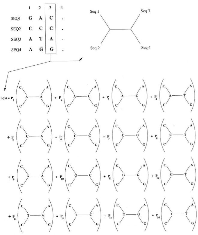
A key assumption of ML is that different alignment positions evolve independently. A second assumption is independent evolution of different lineages. Then, the total likelihood of the tree for the whole alignment is the product of the likelihoods of the individual nucleotides, \(L_{i}\):
The important step is to calculate the likelihood for the individual nucleotides. To do this, all possible trees for a single alignment position are considered. In the case of a sequence alignment with four sequences, this is 16 different trees (Figure 8). The probabilities are calculated by using an evolutionary model of sequence evolution that gives probabilities of mutations between the different nucleotides of a tree. The evolutionary model results in a matrix that describes the mutation probabilities between the four nucleotides. One example of such a matrix is shown in the following table.
| A | C | G | T | |
| A | 0.7 | 0.1 | 0.1 | 0.1 |
| C | 0.1 | 0.7 | 0.1 | 0.1 |
| G | 0.1 | 0.1 | 0.7 | 0.1 |
| T | 0.1 | 0.1 | 0.1 | 0.7 |
This matrix is used to calculate the probability that the four observed nucleotides result by mutation from the 16 possible ancestral configurations. The following steps are taken for calculating the total probability of a tree:
Note that the maximum likelihood procedure for reconstructing phylogenetic trees explicitly assumes a model of evolution to calculate the matrix of mutation probabilities (e.g., the PAM-1 matrix for protein sequences or the Jukes and Cantor model for DNA sequences).
Therefore, the quality of the tree will depend on how biologically realistic the model of evolution is. ML methods are computationally very expensive, but many computer programs were developed that allow to calculate ML trees efficiently. The maximum likelihood method is able to estimate tree lengths. The best and most widely used methods for phylogenetic inference such as IQ-TREE3 are based on Maximum Likelihood.
3 http://www.iqtree.org
Bootstrapping is a technique commonly used for estimating statistics or parameters when the distribution is difficult to derive analytically, i.e., with an explicit mathematical expression (Efron and Tibshirani, 1991). For example, phylogenetic inference from data in the following table results in a tree in which A and B are children of one ancestor and C and D are children of one another.
| Taxon | 1 | 2 | 3 | 4 | 5 | 6 | 7 | 8 |
|---|---|---|---|---|---|---|---|---|
| A | G | C | A | G | T | A | C | T |
| B | G | T | A | G | T | A | C | T |
| C | A | C | A | A | T | A | C | C |
| D | A | C | A | A | C | A | C | T |
It is interesting to obtain a measure of confidence that A and B belong together and that C and D belong together.
Bootstrapping creates pseudo-samples by choosing a site at random and placing it in column 1. This sampling with replacement process is repeated until the number of random columns generated equals the number of sites in the original sequences. Note that because of the sampling with replacement a given column can be sampled repeatedly and each pseudo sample likely omits different columns from the original alignment as shown in the following table, where columns 5 and 1 have been sampled twice each.
| Taxon | 1 | 2 | 5 | 4 | 5 | 6 | 1 | 8 |
|---|---|---|---|---|---|---|---|---|
| A | G | C | T | G | T | A | G | T |
| B | G | T | T | G | T | A | G | T |
| C | A | C | T | A | T | A | A | C |
| D | A | C | C | A | C | A | A | T |
After sampling, the pseudo-sample is used to construct a tree, and for each node in the original tree it is checked, whether it also is present in the bootstrapped sample. The whole process of bootstrapping and analysis of the bootstrapped samples is repeated many times (usually \(>1,000\) times). The confidence for each pair clustering together (i.e., A clustering with B) is then the fraction of times they appear together in the trees generated from many pseudo-samples.
A bootstrap value of 95 then indicates that in 95% of the pseudo-samples OTUs A and B are clustered together, which is quite a good support. For robust inference, bootstrapping requires hundreds or thousands of samples.
The choice of the four very different approaches presented above4 for solving the same problem makes it necessary to select between methods. There is no objective criterion which method to choose, and there have been almost religious wars between the adherents of the different approaches, in particular between ML and Bayesian phylogenicists. One can, however, follow a pragmatic approach:
The phylogeny of the rye genus Secale was calculated using AFLP markers and the UPGMA method (Figure 9). Numbers on branches indicate percent bootstrap support. For interpretation, the taxon Secale cereale is domesticated rye, or other species are either the ancestors or crop wild relatives (CWR) of domesticated rye.
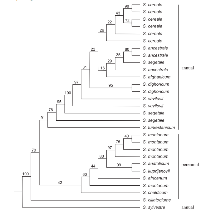
The tree provides several insights:
The phylogeny is based on 160,000 SNP markers that were detected by microarray hybridizations (Figure 10). The three major groups of rice (indica, japonica, austral) are shown in different colors. The tree was reconstructed with an unweighted neighbor-joining method.
Note that bootstrap values (or another measure of statistical support) is not shown, but the branch lengths are indicated.
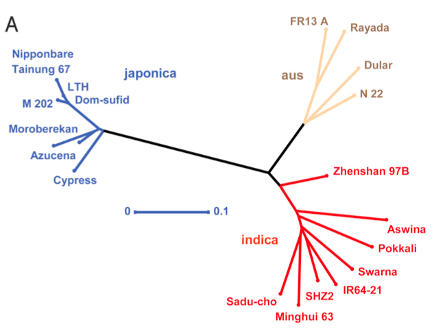
The tree shows that the three major groups of rice are well separated, i.e., have an independent phylogenetic history, and that the aus and indica groups are more closely related with each other.
Books:
Articles:
Search for the figure Figure 10 of this handout in the paper of McNally et al. (2009) and try to find out what a distance of 0.1 means in this figure.
Consider the following distances, based on the allele sharing distance, between different accessions of maize landraces BKN* and wild teosinte TIL* from a paper on maize evolution.
Based on the first 10,000 SNPs in a 3 Mb region
| BKN009 | BKN029 | TIL01 | TIL07 | |
| BKN009 | ||||
| BKN029 | 0.08 | |||
| TIL01 | 0.33 | 0.34 | ||
| TIL07 | 0.21 | 0.20 | 0.37 |
Based on the 30,001th - 40,000th SNPs
| BKN009 | BKN029 | TIL01 | TIL07 | |
| BKN009 | ||||
| BKN029 | 0.11 | |||
| TIL01 | 0.32 | 0.34 | ||
| TIL07 | 0.21 | 0.21 | 0.25 |
Reconstruct the phylogeny of the OTUs using the UPGMA method.
Review the following technical terms which are important when describing and discussing a phylogenetic tree: branch, node, leave, OTU, unrooted phylogeny, rooted phylogeny, clade (monophyletic, paraphyletic, polyphyletic).
Phylogenetic trees are usually expressed in the Newick format which is computer-readable. 1. Write the phylogenetic tree drawn by the instructor in Newick format. Is an alternative possible? 2. A phylogenetic tree is given in Newick format: ((((X,D),F),(S,Y)),W). Draw the tree.
You may want to search the web for a formula that allows to model the number of possible trees given a number of taxa.
Phylogenies are often not that straightforward to read and interpret. In this exercise you will investigate some phylogenies from scientific publications in order to familiarise yourself with them.
Examples for studies that used phylogenetic methods in the context of plant genetic resources:
You will work in groups. Each group is given a phylogeny from a scientific publication. Afterwards you will present your findings to the other groups.
Note: There is no need to read the publication. It is enough to skim through it to collect the relevant information. Also, it is very possibly that not all information is given.
Answer the following questions: - What is shown in this phylogeny? What data was used? - Which method was used to make this phylogeny? Which software was used? - Is it a rooted or an unrooted phylogeny? - Did the authors use an outgroup sequence? - Are the genetic distances shown, i.e. the branch lengths? - Are there any bootstrap values and if yes, how well do they support the nodes? - Is there any clustering of samples? If yes, which are the clusters, how many are there and are all samples in clusters? - Try to interpret and discuss the phylogeny (e.g. which samples are ancestral, which ones are derived).