Selection tests
Motivation
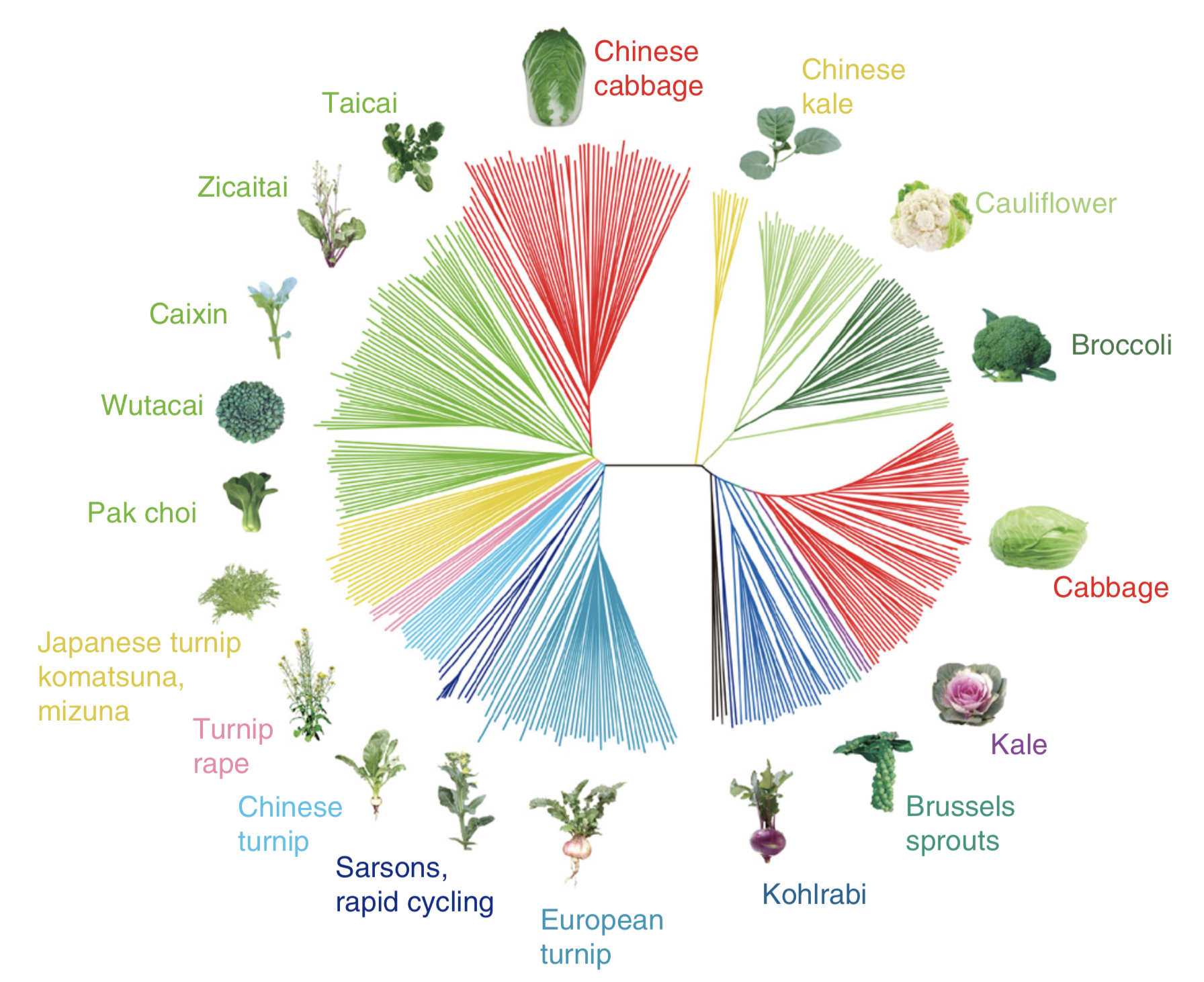
The diversity of crops and landraces is the result of artificial selection by humans. Over time, the selection of favorable traits leads to the enrichment or fixation of genes, which control these traits, in the population. One example are different crops from the two species Brassica rapa and Brassica oleracea. From these two closely related wild ancestors humans selected multiple vegetable crops, which differ by their phenotypic properties (Figure 1)
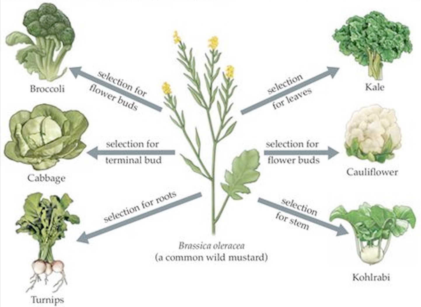
For example from the wild mustard Brassica oleracea cauliflower developed from the selection of flower buds, whereas kohlrabi evolved by the selection of the stem (Figure 2).
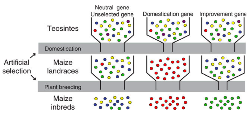
Our knowledge of selection during domestication and modern plant breeding has led to the concept that different genes are selected and fixed at different stages of crop evolution. Figure 3 shows a modification of the original concept by Tanskley and McCouch of different funnels influencing genetic diversity.
Genes or genomic regions, which do not control phenotypic traits under selection, remain polymorphic because only genetic drift and bottleneck effects but not selection influence their diversity. In contrast, genes controlling domestication traits are fixed early in crop evolution and remain monomorphic (i.e., lack genetic diversity) because they continue to be selected. New mutations, which occur rarely, are removed by selection. A third group of genes are improvement genes, which contribute to agronomic properties and they are selected in modern plant breeding programs. These genes differ from domestication genes and they are diverse among landraces, but strongly selected in modern breeding material and varieties and devoid of variation.
Genes controlling phenotypic traits can be identified by two approaches:
- Genetic mapping
- Parents that differ in interesting phenotypic traits are crossed. In the resulting offspring genomic regions controlling these traits are identified by QTL mapping. In genetically diverse material, genome-wide association studies (GWAS) can also be conducted to identify marker-trait associations.
- Selection scans
- This approach scans the genome for regions with unusual patterns of genetic variation using so-called tests of selection. The function of genes with a signature of selection is then further investigated using mutagenesis or genome editing.
Genetic mapping starts with the phenotype of interest, whereas selection scans start with genetic diversity and is agnostic with respect to the phenotype.
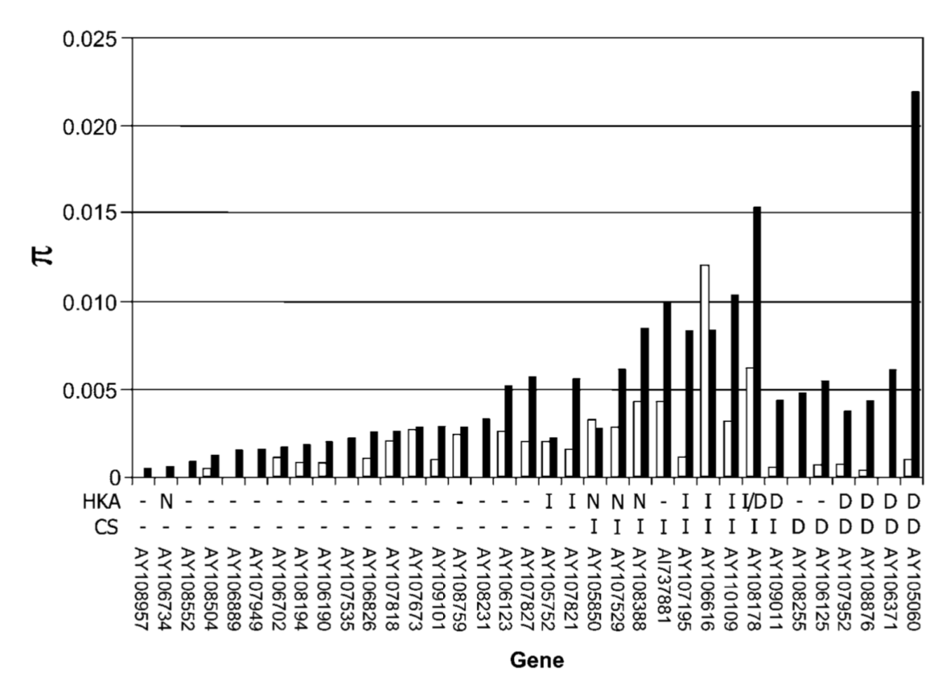
One example is shown in Figure 4, where genetic diversity in modern breeding material, landraces and the wild ancestor of maize were compared in hundreds of genes and those genes identified, which had no genetic diversity in modern material. Several of these genes were known to control traits that are selected in modern breeding programs.
Generally, an analysis of genetic variation in the context of plant genetic resources is useful to determine the patterns and levels of genetic variation in genes and genomic regions of interest for plant breeding, and to identify patterns of genetic relationships in genetic resources. Knowledge about patterns of genetic variation helps to
- identify groups of genetically distinct individuals for breeding (core collections)
- find geographic regions with high levels of genetic variation, for additional collections of genetic resources
- identify suitable populations for introgression into modern breeding populations
- establish heterotic groups for hybrid breeding programs
- estimate the number of accessions in a gene bank collection that need to be sequenced to identify nearly all alleles segregating at a locus (allele mining)
Molecular population genetics is concerned with the genome-wide analysis of observed genetic variation. This branch of population genetics developed in the 1960s with the invention of techniques such as gel electrophoresis that brought about the possibility of monitoring genetic variation within and between species, and to characterize evolutionary forces such as selection, recombination and genetic drift. The rapid progress of DNA sequencing technologies allows the resequencing of the complete genome of numerous genotypes and the characterization of genome-wide genetic variation.
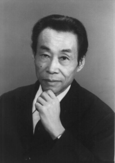
The basic theory of molecular population genetics is the Neutral theory of molecular evolution, which was mainly developed by the Japanese scientist Motoo Kimura (Figure 5). The theory states that the majority of polymorphisms segregating in a population are neutral and have no fitness effects. This statement is based on two main assumptions:
- Strongly advantageous mutations are fixed rapidly in the population and therefore do not segregate.
- Strongly deleterious mutations are removed rapidly in the population and therefore do not segregate.
The neutral theory allows simple and testable predictions of expected patterns of genetic variation in a population. For this reason, the neutral theory is frequently used as a null hypothesis in tests of natural selection.
Application of the theory
A key feature of the neutral theory of molecular evolution (often called neutral model) is that it allows simple predictions.
Assume that you want predict the expected of level of genetic variation at a locus under the neutral model using a sample of \(n\) sequences. Remember that \(\theta = 4N_e\mu\) is the scaled (by population size) mutation rate. Let \(S\) be the number of segregating sites and \(\Pi\) the number of mismatches per pair of sequences. The expected values can be computed from coalescent theory, \[\begin{equation}\label{thetadef} E(S)=\theta\underbrace{\sum_{i=1}^{n-1}i^{-1}}_{:=a_n} \end{equation}\] and \[\begin{equation}\label{thetadef2} E(\Pi)=\theta \end{equation}\] Since \(S\) and \(\Pi\) can be observed in a sample, estimates \(\theta_S=S/a_n\) (Watterson’s estimator) and \(\theta_\Pi=\Pi\) (Tajima’s estimator; note that \(\theta_{Pi}\) and \(\pi\) are the same) can be calculated.
Other properties of genetic variation like the expected site frequency spectrum of polymorphisms can also be derived under the neutral theory.
Types of natural selection
In the analysis of genetic polymorphisms, three major types of natural selection are distinguished:
- Purifying or negative selection
- With this type of selection, deleterious mutations are removed from the population. This is likely the most frequent type of selection because most new mutations are assumed to be deleterious.
- Directional selection
- It causes the replacement of alleles with a new advantageous mutation. This type of selection is also called positive or Darwinian selection.
- Balancing selection
- It is observed if more than one allele of a locus is advantageous. As a consequence, two or more alleles are maintained by selection at a locus.
These different types of selection leave different footprints of genetic variation in the genome and therefore can be differentiated from each other, and also from neutral evolution.
Each type of selection leaves a different footprint of genetic variation in the genome, and tests of selection identify these footprints by analysing patterns of polymorphisms.
Outline of a selective sweep
In the following, we describe a model for the fixation of a new, advantageous mutation by selection, or a selective sweep. During a sweep the following parameters change:
- Level of genetic diversity
- Changes in allele frequencies
- Extent of linkage disequilibrium (LD)
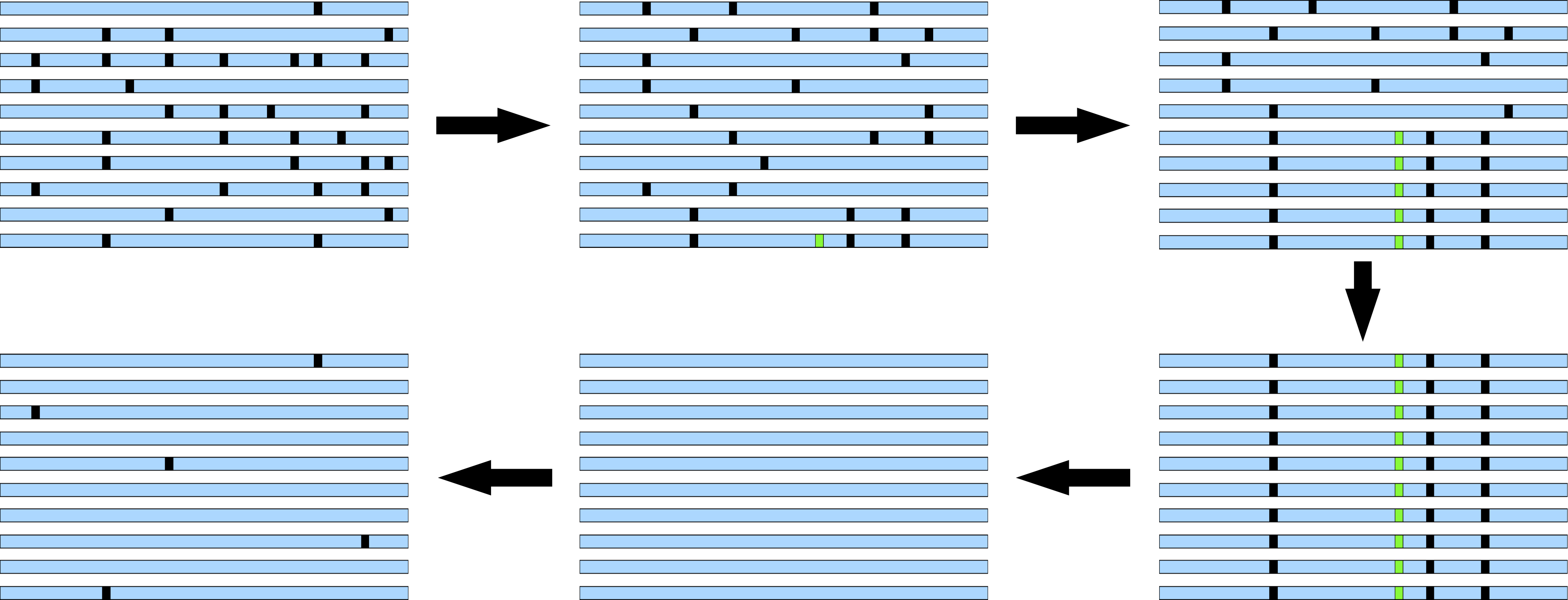
Figure 6 shows a typical selective sweep and shows that a sweep can be divided into several stages:
- Early stage: Intermediate, "normal" LD
- Intermediate stage: Strong LD, high proportion of derived polymorphisms, strong differentiation between haplotypes of ancestral and derived (selected) polymorphism
- Final stage: Lack of polymorphism, very strong LD
- After sweep: Excess of rare polymorphisms
Discussion questions
- How does a selective sweep influence the diversity statistics \(\Pi\) and \(P\)? Are they influenced differently?
- Are there other genetic/demographic mechanisms which could cause a diversity pattern resembling a selective sweep (in the sweep region)?
The “genomic neighborhood” of a sweep
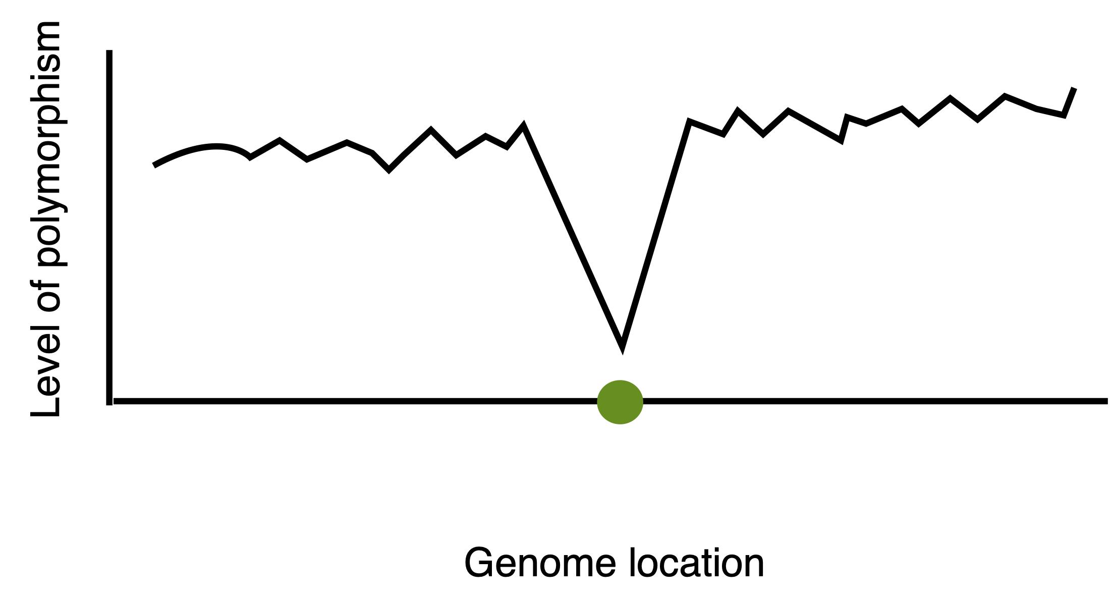
Differences in genetic diversity throughout the genome can be investigated with a sliding window approach. With this method, regions with a strongly reduced level of neutral polymorphism in a region can be detected (Figure 7). The length of the window with reduced variation depends on
- the rate of recombination, \(c\)
- the strength of selection, \(s\)
- How does a high recombination rate affect the window size of low polymorphism?
- How does a high selection coefficient affect the window size of low polymorphism?
- How does the level of linked polymorphisms look with balancing selection?
Tests of neutral evolution
There are several types of neutral evolution, but they all have in common that the null hypothesis is a model of neutral evolution that assumes that no selection occurred in a population. Several tests of neutral evolution were developed to analyse whether the observed patterns of genetic variation have been influenced by non-neutral evolution (i.e., selection). Tests are differentiated by the types of polymorphisms that are investigated:
- Polymorphisms within species (e.g. Tajima’s \(D\))
- Polymorphisms within and between species (e.g. HKA-test)
- Synonymous and nonsynonymous polymorphisms, and synonymous and nonsynomyous substitutions between species (e.g. McDonald-Kreitman-Test)
- Synonymous and nonsynonymous substitutions between species (e.g. \(d_N/d_S\) ratios)
In the following the widely used Tajima’s \(D\) statistic is further described.
Tajima’s D
Tajima’s \(D\), one of the simplest tests of natural selection, is based on different estimators of the population mutation parameter \(\theta = 4N\mu\).
As we already discussed, it was shown by Watterson (1975) that \(\theta\) can be estimated with an infinite sites model as \[\begin{equation}\label{thetawatterson} \hat{\theta}_S=\frac{S}{a_n} \end{equation}\] with \(S\) as the number of polymorphisms at a locus and \[a_n=1+\frac{1}{2}+\ldots+\frac{1}{n-1}\] as a constant that contains the sample size. In an infinite sites model, each mutation hits a different nucleotide position. For this reason, there are only two alleles at each polymorphic site, which is the case for the vast majority of single nucleotide polymorphisms. Tajima (1983) showed that \(\theta\) can be estimated from the nucleotide diversity, \(\pi\), as \[\begin{equation}\label{thetapi} \hat{\theta}_\Pi=\pi L=\Pi \end{equation}\] with \(L\) as the sequence length. The two estimators differ in one important property: \(\theta_S\) depends only on the number of segregating (i.e., polymorphic) positions in the sample, whereas \(\theta_{\Pi}\) is also affected by the relative frequency of the polymorphisms. If there is no selection at a locus, both estimators should give the true value \(\theta=4N\mu\) , hence \(\theta_{\Pi}=\theta_S\) (Tajima, 1989). If one locus evolves under non-neutral evolution, both estimators are affected differently and this information can be used to identify the type of selection.
If an advantageous mutations is fixed by directional selection, linked but neutral polymorphisms also go to fixation by a process called genetic hitchhiking. As a consequence, the level of polymorphism is reduced. After such a selective sweep, new polymorphisms arise by new mutations, which initially segregate at low frequencies in a population (Figure 6). Therefore, some time after the completion of a selective sweep, an excess of rare polymorphisms is expected at a locus. Since \(\theta_S\) depends only on the number of polymorphisms at a locus, it is not influenced by the frequency of the polymorphisms. On the other hand, polymorphisms of low frequency have little effect on the \(\theta_{\Pi}\) estimator. For this reason \(\theta_{\Pi}\) is lower than \(\theta_S\) (\(\theta_{\Pi}<\theta_S\)).
A similar pattern is expected with purifying selection because disadvantageous alleles are removed from the population and therefore occur at a lower frequency in the population than neutral polymorphisms. If there is balancing selection, polymorphisms are retained at intermediate frequencies in the population, and for this reason, \(\theta_{\Pi}\) is expected to be larger than \(\theta_S\) (\(\theta_{\Pi}>\theta_S\)).
Tajima’s \(D\) is then calculated as \[\begin{equation}\label{tajimad} D=\frac{\theta_{\Pi}-\theta_S}{\sqrt{\hat{V}(\theta_{\Pi}-\theta_S)}}, \end{equation}\] which represents the standardized difference of both estimators. Under neutral evolution, \(D=0\), after a selective sweep and during purifying selection, \(D<0\). Under balancing selection, \(D>0\).
The null hypothesis of the test of selection is then \(H_0: D=0\). Now it has to be tested whether the observed value of \(D\) at a locus differs significantly from \(D\), which can be tested with coalescence simulations of several thousand values of \(D\) under a neutral model. For these simulations, only the sample size and the number of observed polymorphisms is needed. Subsequently, a frequency distribution of simulated \(D\) values is generated and the critical values that describe the outer 5% of the distribution are identified. If the observed value is located in the outer 5% of the distribution, the difference from the neutral model is considered to be significant and the hypothesis of a neutral evolution at a given locus is rejected.
This test is shown using an example of the white locus from the fruit fly Drosophila melanogaster using RFLP (Restriction fragment length polymorphism) data (Table 1)
| Type of polymorphism | \(S\) | \(\hat{\theta_S}\) | \(\hat{\theta_\Pi}\) | \(D\) |
|---|---|---|---|---|
| RFLP | 53 | 11.21 | 11.92 | 0.213 |
| Small insertions/deletions | 40 | 8.46 | 10.02 | 0.607 |
| Large insertions/deletions | 15 | 3.17 | 0.94 | -2.071 |
The \(D\) values for the RFLP polymorphisms and the small insertions/deletions (indels) are close to zero, whereas the value for the large indels are highly negative. However, it has to be tested whether this value differs significantly from \(D=0\).
To summarize, a Tajima’s \(D\) value that is significantly lower than expected under neutrality (\(D=0\)) may originate from three causes:
- Selective fixation of advantageous mutations ("selective sweep"): After the fixation of an advantageous allele and the removal of most genetic variation at a locus, new mutations arise that segregate initially at a low frequency.
- Background or purifying selection: Deleterious alleles and any polymorphisms that are linked to it are dragged towards a lower frequency by selection.
- Demographic history: Recent population growth, presence of a migrant individual or strong self-fertilization can all contribute to a significantly negative Tajima’s \(D\).
On the other hand, a Tajima’s \(D\) value that is significantly higher than expected under neutrality (\(D=0\)) may originate from these causes:
- Balancing selection: Multiple alleles are maintained in the population which segregate at intermediate frequencies; special cases include heterozygote advantage, frequency-dependent selection, and also spatial variation
- Demographic history: Population shrinkage or population substructure can result in a signifcantly positive Tajima’s \(D\)
All causes together can cause a significant deviation of Tajima’s \(D\) statistic from the expected neutral value. For this reason, if it has been shown that the observed value is significantly different, further analyses are required to test which of the processes is mainly responsible for the observed pattern.
Coalescent simulations
The critical values for a significant difference of expected and observed values of \(D\) can be obtained with coalescent simulation. For this, several thousand simulated samples with the same number of alleles (\(n\)) and polymorphisms (\(S\)) are generated.
The following is an example of a simulation of 10 chromosomes with a \(\theta = 10\).
ms 10 1 -theta 10
59243

//
segsites: 15
positions: 0.0125 0.1566 0.2156 0.2630 0.3059 0.3209 0.3631 0.3861 0.4501 0.4708 0.7044 0.7493 0.8514 0.9352 0.9356
101000110000110
101000000010011
000000000100000
101010000001010
000001001000000
101000000000010
101010000001010
111100000000010
000000001000000
101100000000010
From these simulated samples, the expected distribution of Tajima’s \(D\) values is generated The value segsites gives the number of polymorphisms, the line positions gives the relative positions of the polymorphisms in the sequence. They are distributed randomly. The 0 and 1 characters are the simulated polymorphisms from which Tajima’s \(D\) is calculated. The expected distribution fo Tajima’s \(D\) with \(n=64\) and \(S=15\) (which corresponds to the values of the large indels in Table 1) for 10,000 simulations is shown in Figure 8.
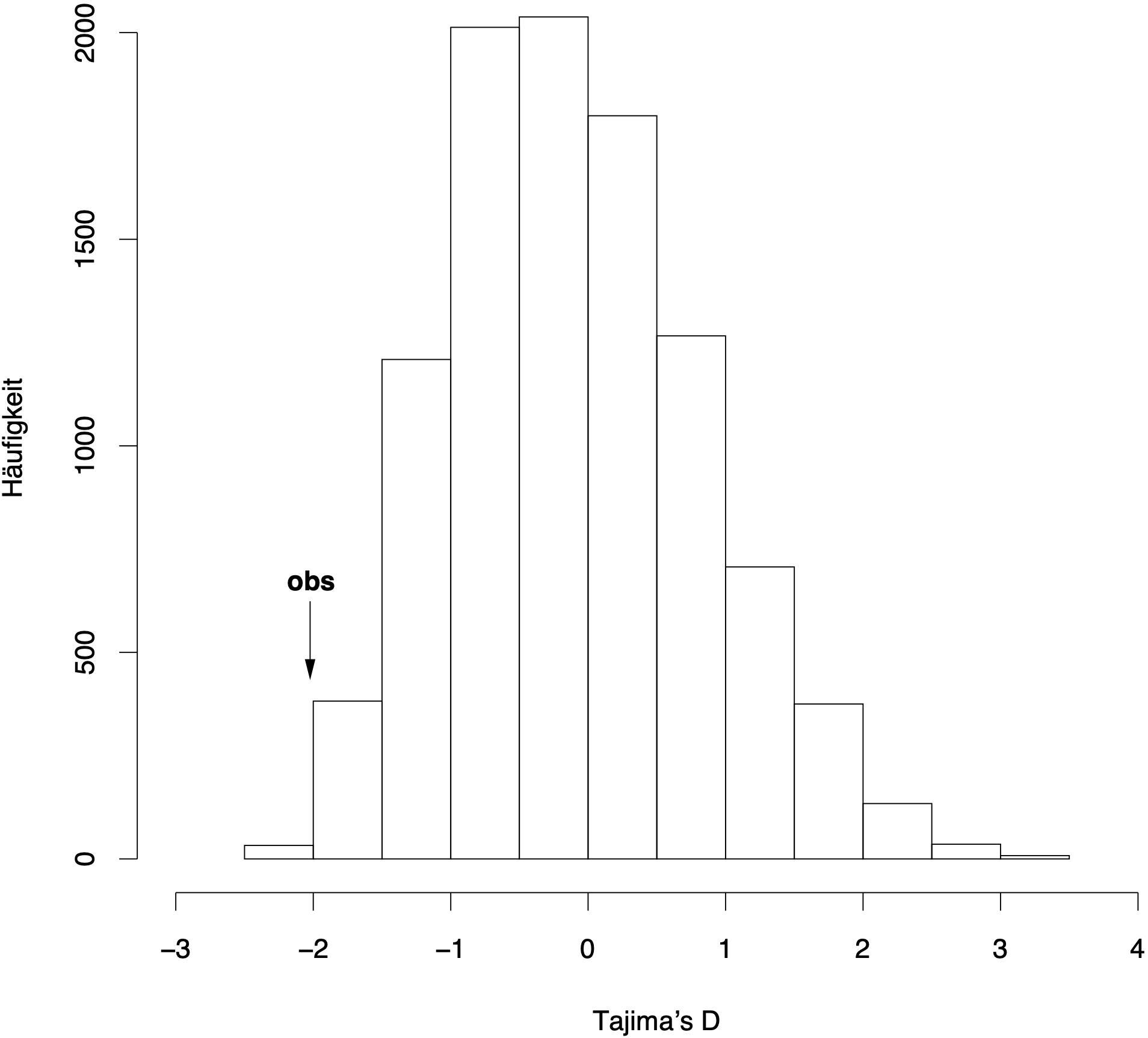
There are two possibilities to test for significance. In a one-sided test one investigates whether the observed value is larger than the one from a null hypothesis. In this case, the critical values are obtained from the right edge of a simulated distribution that covers the outer 5% of the distribution (95% percentile). If one wants to test whether the observed value is significantly smaller than the observed one, the left margin of the distribution is used (5% percentile).
Alternatively, a two-sided test tests whether the observed value differs significantly from the expected value, irrespective of the direction. In this case the critical values are calculated for the left 2.5% and the right 2.5% of the distribution and a subsequent test of whether the observed value is located in these regions.
In our example, the observed values for the large indels (\(D=-2.071\)) is smaller than the 2.5% percentile of the simulated distribution (\(D=-1.66\)) and therefore can be considered as significantly different from \(D=0\) in a two-sided test.
| Polymorphism | Observed | 2.5% Percentile | 97.5% Percentile |
|---|---|---|---|
| RFLP | 0.213 | -1.618 | 2.172 |
| Small indels | 0.607 | -1.672 | 1.758 |
| Large indels | -2.071 | -1.400 | 2.539 |
- Why do coalescent simulations produce a distribution of Taima’s \(D\) values and not the same value in all simulations?
- Observe Tajima’s \(D\) at many loci. How can it be explained if a large proportion of values deviates from the null distribution?
Interpretations of deviations from the null hypothesis
The interpretation of tests of neutrality needs to consider that not only natural selection but other evolutionary processes as well affect patterns of genetic diversity and the statistics that describe this variation. These processes include variation in recombination rate between genes, the presence of a population structure and past changes in population size. The latter two processes, in addition with rates of outcrossing are frequently summarized as the demographic history of a species.
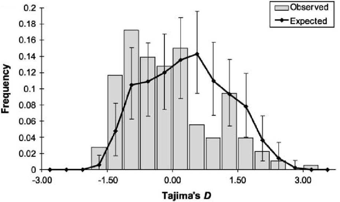
For example, are rapid population growth in the past leads to gene genealogies with long terminal branches. In this case, an excess of rare polymorphisms and a negative value of Tajima’s \(D\) is expected (Figure 9). Since all loci of a genome are affected in a similar fashion from population growth, one expects a negative value for Tajima’s \(D\) for most loci in the genome. By comparing multiple loci with a particular locus, on can determine whether the pattern of genetic variation at a locus differs significantly from the rest of the genome and therefore results from selection. In Arabidopsis thaliana, there is a significant deviation from the neutral standard model (no population structure and population growth, random mating).
Menawhile, similar studies were also conducted in other plant species (Table 2).
| Species | Accessions | Loci | Length | \(\pi_S\) | Tajima’s \(D\) | \(P\) Value | Reference |
|---|---|---|---|---|---|---|---|
| Arabidopsis thaliana | 96 | 846 | 583 | 0.007 | -0.8 | * | Nordborg et al. (2005) |
| Arabidopsis thaliana | 12 | 185 | 414 | 0.010 | -0.4 | * | Karl J. Schmid et al. (2005b) |
| Arabidopsis lyrata | 140 | 77 | 530 | 0.0135 | 0.32 | * | Ross-Ibarra et al. (2008) |
| Boechera drummondii | 46 | 86 | 591 | 0.0041 | -0.46 | Song et al. (2009) | |
| Inbred Maize | 14 | 774 | ? | 0.04 | n.s. | Wright et al. (2005) | |
| Teosinte | 16 | 774 | ? | -0.50 | * | Wright et al. (2005) | |
| Sorghum bicolor | 16 | 204 | 671 | 0.0038 | -0.08 | Hamblin et al. (2006) |
If the standard neutral model is violated, a modified null model must be used that incorporates the particular demographic history of a species to obtain genome-wide distributions of test statistics.
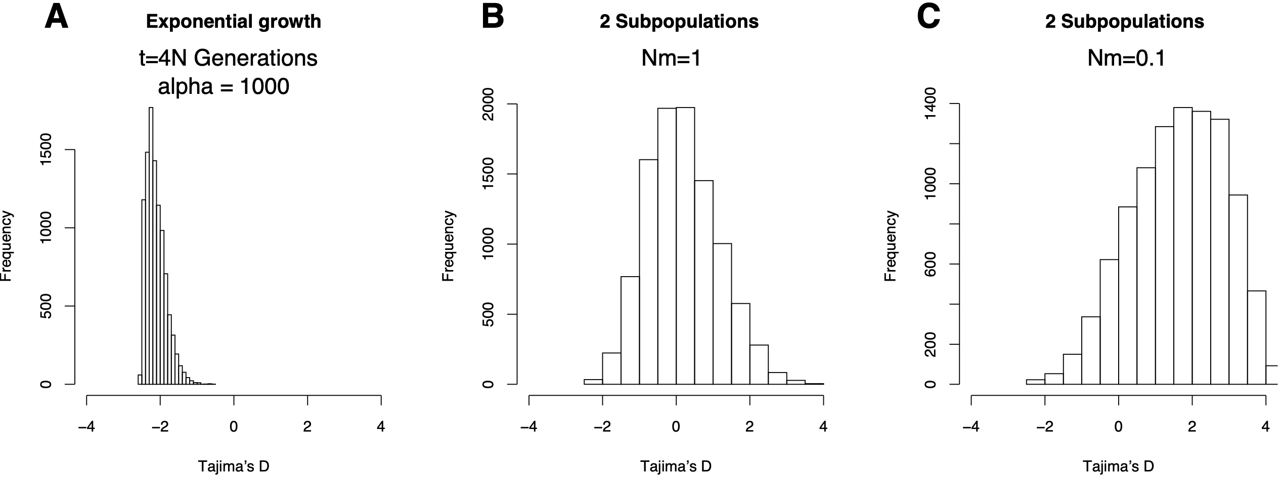
Figure 10 shows simulated distributions of Tajima’s \(D\) under the assumption that the sample size in the past increased exponentially or that the population from which the sample was taken is subdivided into two equal subpopulations with different migration rates between the populations (\(Nm=0.001\) und \(Nm=1\)). The parameter \(Nm\) corresponds to the number of migrants per generation.
The three models are defined by the following parameters:
- Growth rate: \(N(t) = N_0\text{exp}^{-\alpha t}\), \(t\) is the time before present, measured in units of \(4N_0\) Generations
- \(N(t)\) Population size in the past, \(N_0\) current population size
- Two populations which exchange \(Nm\) alleles per generation
To summarize, coalescent simulations are an important tool in the study of genetic variation because they allow the testing of evolutionary hypotheses regarding the history of a sample. In the recent past, coalescent simulations were used mainly for investigating basic population genetic questions, but they are now increasingly used to address more applied questions such in the context of plant breeding and genetic resources.
Key concepts
| \(\square\) Selective sweep | \(\square\) Tajima’s D statistic | \(\square\) Test of selection |
Summary
- There are three types of selection at the molecular level: Purifing, positive and balancing selection.
- Several tests of neutral evolution were developed that are based on the comparison of nucleotide variation within and between species, and on the comparison of divergence between species.
- Tajima’s \(D\) is an important test for the analysis of selection acting on individual genes. This summary statistic measures the frequency distribution of polymorphisms.
- Coalescent simulations are used to test whether the observed levels of Tajima’s \(D\) and other summary statistics are consistent with the neutral level of sequence variation.
Further reading
- Hartl and Clark, Principles of population genetics, Chapter 4
- Nielsen and Slatkin, An introduction to population genetics, Chapters 6 to 9
- Jensen et al. (2007) , Approaches for identifying targets of positive selection. Trends in Genetics 23:568-577 (2007)
- Walsh (2008), Using molecular markers for detecting domestication, improvement and adaptation genes. Euphytica 161:1-17 - A bit dated, but still useful introduction to the topic
Study questions
- How is Tajima’s \(D\) statistic defined and which properties of genetic variation does it measure?
- How is a test of neutral evolution of a locus conducted with the help of the Tajima’s \(D\) statistic and coalescent simulations?
- Why is the expected \(D\) value of a neutral locus zero?
- How does either a selective sweep or exponential population growth cause a negative Tajima’s \(D\)?
- How does Tajima’s \(D\) change in the different stages of a selective sweep? (See Figure 6)
- How does either balancing selection or recent population admixture cause a positive Tajima’s \(D\)?
- How is it possible to differentiate between selection or demography as causes of non-zero values of Tajima’s \(D\) at a locus?
Problems
- Answer the discussion questions in the text above.
- A large number of tests of selection were developed. In addition to comparing allele frequencies, one general approach is to compare the haplotype length of selected and unselected alleles at a locus. Check out Figures 1 and 6 of the paper by Voight et al. (2006), which implements the Extended Haplotype Heterozygosity (EHH) test and the integrated Haplotype Score (iHS). Describe the key principle of this test of selection in works.
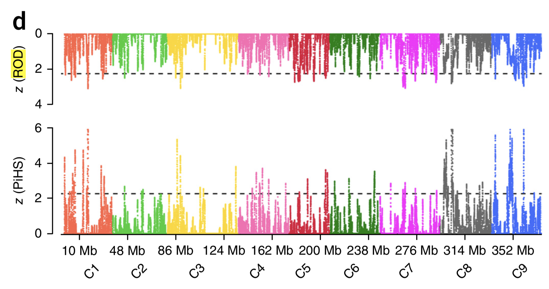
- Figure 11 shows an analysis of diversity (ROH: reduction of diversity) and selection (PiHS, a variant of the iHS test) in Brassica oleracea (Cheng et al., 2016). The statistics were calculated from the resequencing data of all different cabbage types (cauliflower, etc.) in the study. How big is the correspondence between both selection tests? How do you interpret the results with respect to the numbers of genes and genomic regions involved in domestiation of B. oleracea and the subsequent differentiation into crops?
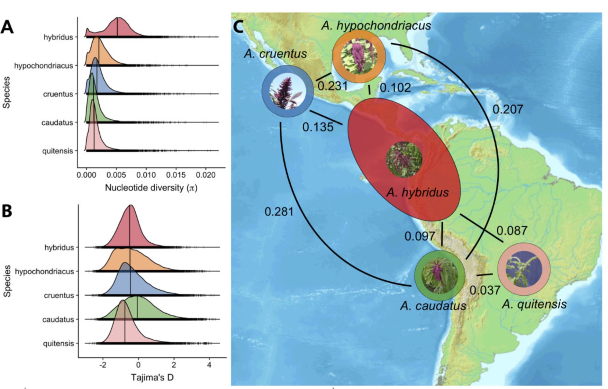
- Figure 12 shows the genome-wide distribution of nucleotide diversity and Tajima’s D of two wild amaranth species (A. hybridus and A. quitensis) and three grain amaranth species (A. caudatus, A. cruentus and A. hypochondriacus). A. hybridus is the ancestor of the three grain amaranth species. What are the difference in nucleotide diversity between domesticated and wild amaranths? What are the values of Tajima’s D between the five groups. Do they fit the expectation of a simple domestication and selection model?