Published

21 Jan 2025

Statistical testing

Motivation

In the previous chapters we derived the basic rules of probability theory from few theoretical foundations and introduced Bayes’ Theorem as an approach to quantify a belief about a scientific hypothesis. We learned that probability theory can be derived from Kolmogoroff’s three axioms.

The goal of this chapter is to make a connection between basic theory of probability and statistical hypothesis testing. Statistical testing can be considered a key component of the scientific method and an essential activity of scientific research. One could even go so far and claim that research scientists are applied statisticians with a domain-specific knowledge (e.g., plant breeding or plant physiology), although such a statement would likely be heavily disputed by a trained statistician.

However, a contrast to trained statisticians is that real scientists are almost exclusively applying statistical procedures that were developed by statisticians, and often do not understand every detail of the procedures they are applying. We referred to this as statistical cargo cult, see here. This situation is somewhat dangerous in research because many statistical procedures and tests make assumptions and every researcher should have sufficient statistical training to understand the nature of these assumptions and the limits of the tests he or she applies in order to avoid wrong conclusions.

The following material therefore is less of a detailed introduction into statistical analysis, but provides an overview of some key concepts in statistical analysis using the scientific method as a framework. You will be introduced to two major approaches to hypothesis testing, Bayesian testing and Frequentist testing.

Learning goals

To understand the connection between probability theory and statistical hypothesis testing, recognizing that statistical testing is an essential part of the scientific method.
To understand the Bayesian and frequentist approaches to hypothesis testing, including their respective foundations and differences, such as the use of prior probabilities in the Bayesian approach and the focus on the null hypothesis in the frequentist approach.
To recognize the significance and types of errors in testing, particularly Type I (false positive) and Type II errors (false negative), and to understand how these errors affect the outcome of hypothesis tests.
To be aware of the replication crisis in science.

Statistical testing and the replication crisis

Closely related to statistical testing is the replication crisis in science (Figure 1). The horsemen are mentioned in the New Testament of the Bible and bring apocalypsis.

The replication crisis refers to the phenomenon where a large proportion of scientific studies are found to be difficult or impossible to replicate. This has led to a growing concern about the reliability and validity of scientific findings, and has prompted calls for reform in the way that scientific research is conducted, reported, and evaluated.

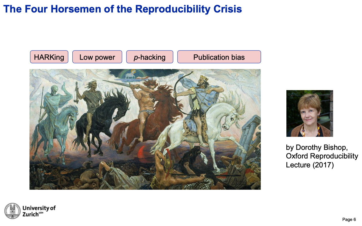
Figure 1: The four hoursement of the replication crisis in science. Source: Leo Heldt, University of Zurich

One contributing factor to the replication crisis is HARKing (Hypothesizing After the Results are Known). This occurs when researchers conduct a study, collect data, and then develop a new hypothesis to fit the data they have collected. This can lead to biased results, as the hypothesis is constructed to fit the data rather than the other way around. It also means that the results of the study are not generalizable to the whole population from which the data (in form of a sample) was collected.

Another major contributing factor to the replication crisis is a low statistical power of studies. Studies with low power are those that have a small sample size, which increases the chances of obtaining false positive or false negative results. Also, the effect sizes (e.g. differences between treated and untreated plants) may be overestimated. In general, studies with a larger sample size have more statistical power to detect effects that are truly present in the population.

$P$-hacking, also known as data dredging, is a related issue where researchers analyze their data and selectively report only results that are statistically significant. This practice can lead to an overestimation of the strength of a relationship or effect and may result in false positive findings. $P$-hacking can take many forms, such as:

testing multiple hypotheses within a single dataset
reporting only significant results
failing to account for multiple comparisons
transforming data to achieve significant p-values
“curating” or “massaging” data (e.g., removing outliers)
collecting data until the desired $p$-value is achieved.

Finally, publication bias is a phenomenon where studies that report positive or statistically significant results are more likely to be published than studies that report null or non-significant results. This bias in the literature can lead to a false impression of the strength of evidence for a given hypothesis.

All of these problems can lead to unreliable and invalid scientific findings, which can have serious consequences for fields such as medicine, psychology, and economics. However, the replication crisis also applies to other fields of science such as crop research. Researchers, funding agencies, journal editors and other stakeholders have been working to address these problems and implement reforms that will help to improve the reliability and validity of scientific research.

Conceptual background

Independent experiments and sampling

We begin the discussion of statistics by introducing the concept of independent experiments and sampling using the classical urn experiments as an example. It should be noted that these experiments can be easily adapted to real scientific situations where discrete units are sampled.

One example is the Hardy-Weinberg Equilibrium in population genetics, which describes the expected frequencies of genotypes (combinations of gene variants in individuals) in a population. Although it makes several assumptions to mimic a simple urn experiment with sampling, it is reasonably close to biological reality and has wide applicability in practical research.

We begin with sampling: Let $\Omega$ be a finite set of objects and $A$ a subset of objects contained in $\Omega$. If we sample (draw) one object at random, the probability of drawing an object from $A$ is: \[\begin{equation} \label{expsampling} P(A)=\frac{\mbox{Number of elements in $A$}}{\mbox{Number of elements in $\Omega$}} \end{equation}\]

We often will denote the number of elements in a set $A$ with $|A|$.

Independence: Two experiments are independent, if for each sets of outcomes $A$ from Experiment 1 and $B$ from Experiment 2 we have \[\begin{equation} \label{expsampling2} P(B|A)=P(B)\Leftrightarrow P(A|B)=P(A) \Leftrightarrow P(A\cap B)=P(A)P(B) \end{equation}\]

Sampling with replacement: Let $\Omega$ be a finite set of objects. If we sample (one element) with replacement, we draw one object at random from $\Omega$ and replace it with an identical object (put it back). Therefore, the probability of sampling objects $1,...,k$ with replacement from sets $A_1,\ldots,A_k$ is \[\begin{equation} \label{expsampling3} P(A_1)\cdots P(A_k) \end{equation}\]

Using an urn experiment and a binomial distribution

We previously derived the notions of a finite set of objects, $\Omega$ and the probability of a subset $A$ from which an object is sampled with a certain probability. The concept of sampling with replacement was also introduced.

These concepts will now be applied to a classical urn experiment, which are frequently used in probability theory to demonstrate a statistical concept.

Consider an urn with red and green balls (or a set of objects $\Omega$ with either trait $A$ or $B$). The frequency of red balls is \[\begin{equation} \label{red} p_{\text{Red}} = \frac{|A|}{|\Omega|}, \end{equation}\]

and the frequency of green balls is \[\begin{equation} \label{green} p_{\text{Green}} = (1-p) = \frac{|B|}{|\Omega|}, \end{equation}\]

We draw a ball $n$ times with replacement. Then, the probability of drawing $k$ red balls and $n-k$ green balls (in any order) is given by the binomial distribution, \[\begin{equation} \label{binomialsampling} P(\mbox{$k$ red balls})=\frac{n!}{k!(n-k)!}p^k(1-p)^{n-k}. \end{equation}\]

In the following we show this with an example calculation.

The setup of an urn is then $p(\text{red ball}) = p(\text{green ball}) = 0.5$.

Figure 2: A urn with a total of 4 balls, of which two are red and two are green.

Figure 3 shows a possible outcome of an experiment with five draws ($n=5$). Note that the order of the colors does not matter in this experiment, only the frequencies.

Figure 3: Possible outcome of a drawing experiment with $n = 5$ draws.

With an urn experiment, on can easily generate a hypothesis to test, produce empirical data and apply a statistical test of a hypothesis. This simple experiment will be used to test a hypothesis using Bayesian inference and frequentist statistics to demonstrate the key differences between both approaches.

Statistics as inductive logic

Before conducting statistical hypothesis tests, we first introduce a few concepts.

Statistics is defined as applied inductive logic. It is inductive (i.e., conclusions are made from the specific to the general), because a sample is used to make a statement about the whole population.

In the case of the urn experiment, the parameters and hypotheses are closely related. Under the assumption that four balls are in the urn that can be either red or green, parameters to be estimated are the numbers of red or green balls. Hypotheses that can be tested are for example that there are 2 red balls in the urn (Hypothesis 1) or 3 red balls in the urn (Hypothesis 2).

In the context of statistical inference it needs to be considered whether a sample size is large enough to make a statement about the whole population, and whether the data are eligible and sufficient for testing hypotheses.

Bayesian statistical inference

Since Bayes’ theorem was already introduced we describe in the following a Bayesian statistical analysis of urn experiment ¹

Example of an urn experiment

We use the following experimental setup.

First randomly decide which of two hypotheses is the true hypothesis, i.e., select the urn.

If ‘head’, place 1 red and 3 green balls in an urn.
If ‘tail’, place 3 red and 1 green balls in an urn.

In other words, chance decides which hypothesis is true, and the goal is to determine using a Bayesian approach to find the correct hypothesis among the two possible hypotheses:

$H_G$: 1 red and 3 green balls (RGGG)
$H_R$: 3 red and 1 green balls (RRRG)

The following approach is taken for the experiment:

Purpose: To determine which hypothesis, $H_G$ or $H_R$, is probably true.
Experiment: Mix the balls, draw a ball, observe its color, and replace it, repeating this procedure as necessary.
Stopping rule: Stop when a hypothesis reaches a posterior probability of 0.999.

Since only two hypotheses are compared, the ratio form of Bayes’ rule can be used: \[\begin{equation} \label{bayexp1} \frac{P(H_G|D)}{P(H_R|D)} = \frac{P(D|H_G)}{P(D|H_R)} \times \frac{P(H_G)}{P(H_R)} \end{equation}\]

Since both hypotheses have equal chance of being true (the coin decided about the correct one), they have the same prior probabilities: $P(H_G) = P(H_R) = 0.5$.

The second term in Bayes’ rule is the likelihood function. For an experiment with a single draw of a ball, the likelihood functions are for the two hypotheses are simply the probabilities to draw a green ball under each of the two hypotheses:

$H_G$ (WBBB): $P(\text{green}|H_G)=3/4=0.75$
$H_R$ (WWWB): $P(\text{green}|H_R)=1/4=0.25$

For an experiment with two draws of a ball (sampled with replacement) they are:

$H_G$ (WBBB): $P(\text{green,green}|H_G)=(3/4)^2=0.5625$
$H_R$ (WWWB): $P(\text{green,green}|H_R)=(1/4)^2=0.0625$

For experiments with $(n+1)$ draws, the posterior odds of the $n$-draw experiment is the prior to a one-draw experiment. In other words, we use the posterior probability of a hypothesis of the previous experiment as the prior probability of the same hypothesis for the next experiment. This demonstrates an important principle of Bayesian statistical inference, namely that it is possible to learn from prior data.

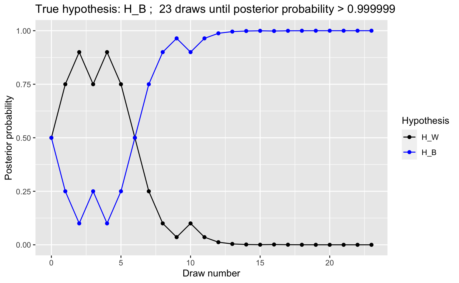
The course of the experiment over different draws is shown in Table 1.

Table 1: Results of 15 draws of a Bayesian analysis of a urn experiment. In each draw the posterior probability of the two hypotheses are used as prior probabilities for the next draw. Source: Gauch (2003)

Draw	Result	Posterior $H_B:H_W$	Posterior $P(H_B \| D)$
	(Prior)	1:1	0.500000
1	White	1:3	0.250000
2	Blue	1:1	0.500000
3	White	1:3	0.250000
4	Blue	1:1	0.500000
5	Blue	3:1	0.750000
6	Blue	9:1	0.900000
7	Blue	27:1	0.964286
8	Blue	81:1	0.987805
9	Blue	243:1	0.995902
10	White	81:1	0.987805
11	Blue	243:1	0.995902
12	White	81:1	0.987805
13	Blue	243:1	0.995902
14	Blue	729:1	0.998630
15	Blue	2187:1	0.999543

Figure 4 show the trajectory of posterior probabilities of one such an urn experiment. It was generated with the R quarto notebook in this link link.

Figure 4: Simulation of an urn experiment and calculation of the posterior probabilities using Bayes’ theorem.

The relationship between the two hypotheses, which are being tested, can be expressed with the following equation \[\begin{equation} \label{bayexp2} \underbrace{\frac{P(H_G|D)}{P(H_R|D)}}_{\mbox{odds ratio}} = \underbrace{\frac{P(D|H_G)}{P(D|H_R)}}_{\mbox{Bayes factor}} \times \underbrace{\frac{P(H_G)}{P(H_R)}}_{\mbox{prior odds}} \end{equation}\]

The odds ratio is the ratio of the posterior probabilities. It answers the question: How many times more probable is $H_G$ compared with $H_R$ given the observed data? If the odds ratio is smaller than 1 (e.g., 0.1), it is convenient to say that $H_R$ is $\frac{1}{\mbox{odds ratio}}$ times more probable than $H_G$ (e.g., $(0.1)^{-1}=10$ times more probable) given the data.

A Bayes factor is then a ratio of the likelihoods. It answers the question: How many times more probable is it to see the data under $H_G$ than under $H_R$?

To summarize, with Bayesian statistical inference, it is possible to compare two hypotheses and with a suitable experimental design (e.g., a sufficient number of draws) and to decide on one of two (or more) hypotheses.

Frequentist statistical inference

Although the Bayesian paradigm preceded the frequentist paradigm by a few hundred years, the frequentist approach is more commonly used today and is considered the ‘standard’ or textbook method for conducting statistical analyses.

One motivation for developing the frequentist paradigm was to eliminate the need for prior probabilities required by Bayes’ theorem, as they were considered a subjective choice. Thus, an important goal of the frequentist paradigm was to make statistical analysis more objective.

Ronald Aylmer Fisher (Wikipedia) was one of the key proponents of frequentist statistics, developing foundational methods that are still widely used today. Jerzy Neyman (Wikipedia) and Egon Pearson (Wikipedia) further developed frequentist hypothesis testing to emphasize the principle of falsification.

The philosophical foundation of the frequentist paradigm was provided by Karl Popper, who proposed that scientific theories need to be falsifiable. This philosophy aligns well with the frequentist paradigm, as it focuses on testing a single hypothesis (the null hypothesis) and provides a framework for accepting or rejecting it.

Most scientists adopted the frequentist paradigm because it was conceptually simpler—focusing on a single hypothesis—computationally more feasible, and more objective, as it does not rely on prior probabilities.

Foundations of frequentist hypothesis testing

Frequentist hypothesis testing focuses on testing a Null Hypothesis ($H_0$). Examples of null hypotheses from the field of crop science include:

: “There is no effect of a treatment on an outcome, such as a herbicide treatment on crop yield.”: “Genotype frequencies at a gene are in Hardy-Weinberg equilibrium in a population.”
Corresponding alternative hypotheses ($H_1$) are then, for example:: “There is a treatment effect, such as a herbicide treatment affecting crop yield.”; “Genotype frequencies at a gene deviate from Hardy-Weinberg equilibrium in a population.”

Note that the exact effect size for the alternative hypothesis does not need to be specified.

Statistical tests are used to either reject or fail to reject the null hypothesis. Only the null hypothesis is directly tested, and it is typically formulated as a specific statement. It is important to note that a hypothesis cannot be accepted and rejected simultaneously.

Hypothesis testing occurs within a clearly defined setup that includes:

A fixed stopping rule (see below), and
Fixed hypotheses (the hypotheses cannot be altered during testing).

Errors in testing

By focusing on accepting or rejecting a null hypotheses, two possibilities for errors are introduced.

A frequentist’s test accepts or rejects the null hypothesis, $H_0$. The decision is based on the sampled data and may not be correct. Two types of errors are possible:

Decision	$H_0$ True	$H_0$ False
Accept	Success	Type II Error
Reject	Type I Error	Success

False Positive (Type I Error): Reject a null hypothesis even it is true.
False Negative (Type II Error): Accept a null hypothesis even it is false.

For example if $H_0$ states “A fungicide does not protect a plant” (Treatment has no effect) the possible errors are:

False positive error (Type I): Conclude that a fungicide protects a plant even it does not ($H_0$ is true)
False negative error (Type II): Conclude that a fungicide does not protect a plant even though it does ($H_0$ is false)

Ideally, a statistical test would completely avoid both errors. However this is not possible, an there is a trade-off between both types of errors.

Any false positive error can be avoided by accepting the null hypothesis in any case.
Any false negative error can be avoided by rejecting the null hypothesis in any case.

Since it is not possible to accept and reject $H_{0}$ at the same time, both of these “extreme” approaches are not useful.

In frequentist hypothesis testing, the solution to this problem is to accept a certain probability $\alpha$ of a false positive (type I) error. This probability is called the significance level, which represents the threshold for rejecting the null hypothesis $H_0$.

A $p$-value is calculated for a statistical test based on the observed data. The $p$-value is defined as the probability of obtaining a result at least as extreme as the observed outcome, assuming that $H_0$ is true. A small $p$-value provides strong evidence against $H_0$, suggesting that it may be rejected.

The $p$ value is calculated by assuming that the experiment is repeated infinite times under the assumption that $H_0$ is true. By comparing the observed test statistic with the repeated experiments, the probability of getting an outcome as extreme or more extreme than actual experimental outcome is used to decide upon the acceptance or rejection of a null hypothesis.

The term frequentist derives from the assumption that the experiment is carried out infinite times to obtain the critical level of significance for accepting or rejecting the null hypothesis.

A frequentist analysis of the urn experiment

We now carry out a frequentist analysis of the null hypothesis. First, we define the hypotheses:

Null hypothesis $H_R$: Three red and one green ball
Alternative hypothesis $H_G$: Any other combination of red and green balls.

Note that we used an arbitrary selection of a null hypothesis! It is important to consider that the choice of a certain $H_{0}$ influences test interpretation. The test does not make any assumption about the prior information (i.e., does not propose an expectation about the frequency of red and green balls in the urn).

Before conducting the experiment and the test, a significance level $\alpha$ is chosen.

The outcome of experiments is described by the test statistic $T=$ number of green draws.

Then, $H_{0}$ is tested by calculating the $p$ value as \[\begin{equation} \label{pvalue} P(T\geq t\mid H_R), \end{equation}\] where $t$ is the actual value of $T$ in the experiment. Reject $H_R$ if $p\leq \alpha$.

We take 15 draws and Table 2 shows the possible 16 outcomes of $T$ with four balls in each experiment.

Table 2: Frequentist analysis for a marble in an urn experiment assuming that the null hypothesis $H_{W}$ is true and the experiment stops at 15 draws. Source: Gauch (2003)

Blue Draws	Probability	p-value
0	0.01336346101016	1.00000000000000
1	0.06681730505079	0.98663653898984
2	0.15590704511851	0.91981923393905
3	0.22519906517118	0.76391218882054
4	0.22519906517118	0.53871312364936
5	0.16514598112553	0.31351405847818
6	0.09174776729196	0.14836807735264
7	0.03932047169656	0.05662031006068
8	0.01310682389885	0.01729983836412
9	0.00339806545526	0.00419301446527
10	0.00067961309105	0.00079494901001
11	0.00010297168046	0.00011533591896*
12	0.00001144129783	0.00001236423850
13	0.00000088009983	0.00000092294067
14	0.00000004190952	0.00000004284084
15	0.00000000093132	0.00000000093132

The following parameters can be calculated: The average of $15 \times 0.25 = 3.75$ draws of green is expected given $H_R$. The exact calculation with $g$ (green), $r$ (red) and $n=g+r$ draws (given $H_R$) is \[\begin{equation} \label{binomialexpectation} p_b=\frac{n!}{b! \times w!} \times 0.25^b \times 0.75^w \end{equation}\]

This calculation follows the binomial distribution. The probability for exactly 5 green and 10 red draws (given $H_R$) is then \[\begin{equation} \label{binomexp} \frac{15!}{5! \times 10!} \times 0.25^5 \times 0.75^{10} \end{equation}\]

If $t$ green draws are observed, p-value is \[\begin{equation} p=\sum_{g\geq t}p_g. \end{equation}\]

This test paradigm is called binomial test.

Table 2 shows that with a number of 0 blue draws ($t=0$) the $p$-value is 1, because the sum of all individual probabilities of 0 or more blue draws is 1, i.e., all values in the second column of Table 2 need to be added up.

The conclusion, marked by an asterisk for the experimental outcome of 11 green draws, is to reject $H_{R}$ at a highly significant $p$ value of 0.000115. This $p$ value means that if experiments with $H_{R}$ were to be conducted numerous times, a result as extreme as 11 green or more green draws would occur with a frequency of only 0.000115, or only in about 1 in 8,700 experiments.

Compare this to the outcome of the Bayesian analysis described in Table 1, where the same number of blue draws were observed and a posterior probability of .9999543 for hypothesis $H_B$ was calculated.

The $p$ values in Table 2 can be interpreted as follows. Assume the in 15 draws there are 8 draws of the green ball. The exact probability to draw 8 balls under $H_R$ is 0.013106. The probability to draw 8 balls or more is 0.01729, calculated as the sum of the individual probabilities for 8 to 15 green draws. This sum is the p-value. If we assign $\alpha=0.05$ we can state that if we draw 8 or more green balls, we reject $H_R$ because $p$-value $<\alpha$.

For a better understanding Figure 5 shows a simulation of this urn experiment. It shows the frequency distribution of green balls in a total of fifteen draws unter the null hypothesis of $H_{R}$ that was repeated one million times. Out of these repetitions, only $92+16+1$ experiments showed 11 or more green balls. Under our null hypothesis the observed outcome is very rare with a frequency of $114/1,000,000= 0.000114$, leading us to reject the null hypothesis of $H_{R}$ and below our significance level of $\alpha=0.05$.

Figure 5: Frequency distribution of the outcome of an urn experiment under $H_0$, i.e., three red and one green ball in the urn ($H_R$ in the text). The experiment of 15 draws was repeated $1^6$ times and the number of green balls was recorded in each experiment. The red line indicates the expectaton value of 3.75 green balls under the null hypothesis $H_{R}$. Julia code for this figure: Link

$p$ values versus effect sizes

A highly significant test result (= very low $p$ value) just gives the information that we can distinguish very well between the null and alternative hypotheses using our inference rule (= test) and our data. However, it does not state whether the difference in the test statistic between the two hypotheses, $H_{0}$ and $H_{1}$, is big or not. In other words, the $p$ value does not tell us something about the effect size (e.g., the difference in outcome between two treatments).

The problem is further exacerbated by the fact that given enough data, even very minor differences between hypotheses can be highly significant. If one expects a small effect size, an increase in the sample size can make a statistical test highly significant. Increasing the sample size until significance is achieved is one approach of $p$-value hacking, which is the practice to ‘adapt’ statistical tests in a manner that they produce significant results, which are then publishable and contribute to the advancement of the careers of scientists.

The relationship between $p$ values and effect sizes is demonstrated in the following example.

Consider two sets of two urns each with green and red balls and certain observed values:

Experiment 1:: Urn A1 has 9 green balls and 1 red ball ($H_1$), urn A2 has 1 green ball and 9 red balls ($H_0$). We drew 3 balls and observed 3 green balls.
Experiment 2:: Urn B1 has 6 green and 4 red balls ($H_1$), urn B2 has 5 green and 5 red balls ($H_0$). We drew 12 times and observed 12 green balls.

The key differences between the experiment is that in Experiment 1 there were only 3 draws and in Experiment 2 12 draws. The $p$ value in in experiment is $p =(0.1)^3=0.001$, and in Experiment 2 $p =(0.5)^{12}\approx 0.00024$.

Since the $p$ value in Experiment 2 is lower than in Experiment 1, there is a lower chance of making a false positive error in the second experiment, although the difference between the hypotheses (the effect size) is much smaller in the second experiment.

Comparison of Bayesian and Frequentist Approaches

The Bayesian and frequentist approaches offer distinct frameworks for statistical analysis and hypothesis testing, each with its own philosophical foundation and practical applications.

Bayesian statistics focus on determining the probability that a hypothesis is true given the observed data and any prior knowledge or beliefs. For example, in a crop yield study, Bayesian analysis would allow you to incorporate prior information—such as past experiments, expert knowledge, or historical yield data—into the analysis. The result is a posterior probability, which provides a direct and interpretable measure of how likely the hypothesis (e.g., “a herbicide increases crop yield”) is true, given both the data and prior evidence. This approach is particularly useful when data are limited or when prior knowledge is available, as it allows researchers to update their beliefs as new evidence emerges.

Frequentist statistics, on the other hand, focus on the reliability of inference procedures by evaluating their performance over repeated experiments. This approach assesses the probability of rejecting a true hypothesis (Type I error) or failing to reject a false hypothesis (Type II error). For example, when testing whether a herbicide has an effect on crop yield, frequentist methods use p-values and confidence intervals to make decisions about the null hypothesis (e.g., “there is no effect”). Unlike Bayesian methods, frequentist analysis does not incorporate prior information and interprets probabilities based on long-run frequencies of repeated sampling under the null hypothesis.

In summary, Bayesian statistics provide a probabilistic interpretation of hypothesis truth by integrating prior knowledge with observed data, while frequentist statistics emphasize the reliability of hypothesis testing procedures based on error rates in repeated experiments. The choice between these approaches often depends on the availability of prior information, the study design, and the goals of the analysis.

Key concepts

Replication crisis in science
HARKing, underpowered studies, $p$-value hacking, publication bias
Probability theory versus statistical inference
Bayesian versus frequentist hypothesis testing
Measures of confidence: Posterior probability versus $p$-value

Summary

In this lesson the comparison between Frequentist and Bayesian inference was based on an abstract ball experiment to demonstrate the key concepts of both approaches. However, even this simple example can be easily translated into a practical setting, for example in the context of the inheritance of alleles.

Bayesian statistics answers the question about probability of hypotheses given data directly. It compares several hypotheses, for which prior probabilities have to be assigned. :::{.content-hidden .comment} - In contrast, it does not need a stopping rule. ::: Bayesian inference has some additional challenges, which were not discussed here, but prevented its widespread adoption. For example, a model is needed to calculate the likelihood of the data given a hypotheses, and for realistic scenarios, this can be a formidable challenge.

Frequentist statistics presents inference scheme which has a certain quality (controlled type I error). It allows to compare hypotheses, but also to test whether a null hypothesis can be rejected without specifying an alternative, because the alternative hypothesis does not need to be specific and only the negation of the null hypothesis ($H=H_0$ vs. $H\neq H_0$). Frequentist hypothesis testing does not need a prior probability for the hypotheses. :::{.content-hidden .comment} , but needs a stopping rule. :::

Both methods are useful, but have different strengths. A key difference is that Frequentist statistics puts the emphasis on the process of inference, whereas Bayesian statistics puts the emphasis on evaluating the support for (multiple) hypotheses.

A good knowledge of the assumptions, methods and conditions of statistical testing is required to make robust inferences about scientific hypotheses and to avoid the problems caused by the replication crisis.

Study questions

List the pros and cons for Bayesian and frequentist statistics
One argument in favor of frequentist statistical analysis was that it is more objective than Bayes’ statistical inference. Where do you see the subjectivitiy in Bayesian inference?
Which of the two statements is true:
A $p$-value indicates the probability that a $H_0$ is false.
A $p$-value gives the probability that an alternative hypothesis $H_1$ is true.
A $p$-value gives the relative frequency of an observed outcome of an experiment is as extreme or more extreme as expected under a $H_0$.
A $p$-value gives the relative frequency of an observed outcome of an experiment is as extreme or more extreme as expected under a $H_1$.
Let us redo the urn experiment with balls. This time, we only draw 4 times and we see the following sample: green, green, green, red. Do a Bayesian and a frequentist’s test for deciding whether this sample gives evidence for $H_R$ or $H_G$. For the Bayesian test, just give the posterior probability ratio, for the frequentist test compute the $p$-value.
We want to test in the frequentist’s way whether a locus is in Hardy-Weinberg equilibrium (HWE) and formulate the hypotheses

$H_0$:	Locus is in HWE
$H_1$:	Locus is not in HWE

What are the possible false positive and false negative errors for these hypotheses? Remark: You don’t have to formulate a test, just describe the possible errors.

References

Eddy SR. 2004. What is Bayesian statistics? Nature Biotechnology 22:1177–1178. doi:10.1038/nbt0904-1177

Gauch HG. 2003. Scientific method in practice. Cambridge University Press.

Gauch Jr HG. 2012. Scientific method in brief. Cambridge University Press.

Krzywinski M, Altman N. 2013. Points of significance: Significance, p values and t-tests. Nature Methods 10:1041–1042. doi:10.1038/nmeth.2698

McElreath R. 2016. Statistical rethinking: A bayesian course with examples in r and stan. CRC Press.

Nuzzo R. 2014. Scientific method: Statistical errors. Nature News 506:150. doi:10.1038/506150a

Puga JL, Krzywinski M, Altman N. 2015b. Points of significance: Bayesian statistics. Nature Methods 12:377–378. doi:10.1038/nmeth.3368

Puga JL, Krzywinski M, Altman N. 2015a. Points of Significance: Bayes’ theorem. Nature Methods 12:277–278. doi:10.1038/nmeth.3335

Footnotes

The example is taken from Gauch (2003)↩︎