Cleaning and processing scientific data

Introduction

This handout is based on the online tutorial https://cran.r-project.org/web/packages/tidyr/vignettes/tidy-data.html and edited by members of the research group Crop Biodiversity and Breeding Informatics (350b), University of Hohenheim.

We will work with four different data files: preg.csv, preg2.csv, preg4.csv, and pew.csv. Download them from our website and save them somewhere where you can find them.

Learning goals

The learning goals of this class is to understand:

• What are messy data?
• What are tidy data?
• How tidy up messy data?
• How to write tidy data into a csv file?

Storage of data

Data can be stored in many ways. Usually, data is stored in spread sheet format in a csv-file. csv stands for ‘comma-separated-values’. Very large data sets are usually stored in data bases. Data bases have the additional advantage that they allow cross-linking and retrieving different types of data. In this class only two dimensional spread sheet data will be considered using a small data set.

It should be noted that small data sets are frequently also in other formats, such as ‘.xlsx’ or ‘.xls’ (Excel) or ‘.ods’ (LibreOffice).

Reading data into R

We start with the data file preg.csv. Import it into R. Note: depending on where you saved the file, you will have to change the path.

```{r}
preg <- read.csv("data/preg.csv", stringsAsFactors = F) # change the path if necessary
# and have a look on its structure 
str(preg)
```

The read.csv function imports csv-formatted data into R and turns them into an R-object of the type data.frame. There are also other read.-functions, like read.table(). Try ?read.table and you will get an overview.

Types of messy data

This is a very short data.frame so we can also directly look at it.

```{r}
preg
```

Alternatively the same data can be stored in a different way (preg2.csv):

```{r}
preg2 <- read.csv("data/preg2.csv", stringsAsFactors = F) # change the path if necessary
preg2
# for comparison:
preg
```

These two files contain the same data set. What is different between the two files?

Different ways of storing the data are requested by different programs/packages. However, some ways of storing your data are more convenient than others. The R package tidyr (Wickham 2016), which is included in the tidyverse package, can convert data in several ways to easily generate the optimal data structure for data analysis.

For instance with the former two presentations of the data we can not easily make a meaningful plot or analysis. This is why the authors of tidyr call this type of data storage “messy”.

What is tidy data?

There are three interrelated rules which make a data set tidy:

1. Each variable must have its own column.
2. Each observation must have its own row.
3. Each value must have its own cell.

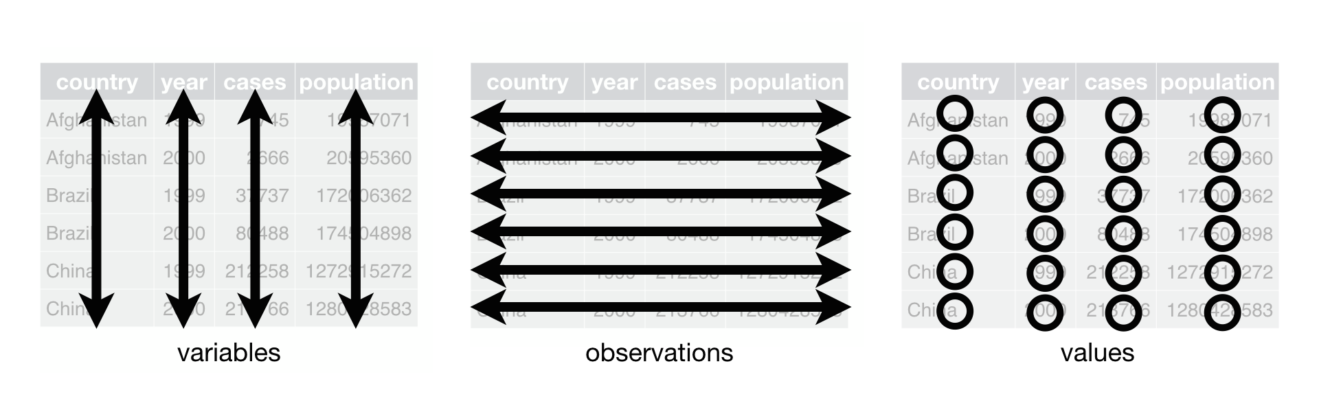{#fig-tidydata width=80%}

The tidyverse set of libraries have functions to convert data into a tidy format. They are used in the following code junk. Note that the pipe operator %>% is used which binds different functions as if in one line.

Cheat sheets

To be familiar with tidyverse, you can read the cheat sheets from the RStudio website (https://www.rstudio.com/resources/cheatsheets/). For this computer lab tutorial, you may look at:

• A cheat sheet of dplyr (Click here to download)
  
• A cheat sheet of tidyr (Click here to download)

Help and R documentation

For the most of R functions, you can access a user manual that gives a description of the function and possible arguments. For instance, if you can get help on read.table with ?read.table or help(read.table).

How can we use tidyverse to make our messy data tidy?

First, we load the tidyvers package (if it is not installed yet, install it using install.packages("tidyverse")):

```{r}
library(tidyverse)
```

Then run the following code to tidy the data:

```{r}
preg3 <- preg %>% 
  gather(treatment, n, treatmenta:treatmentb) %>%
  mutate(treatment = gsub("treatment", "", treatment)) %>%
  arrange(name, treatment)
```

Now each observation is a row, each variable (including the treatment) is a column and the columns are sorted by subject, which is in this case “name”.

```{r}
preg3
# or
str(preg3)
```

In this format, it is easy to make a boxplot of the data:

```{r}
par(mfrow=c(1,2))
boxplot(n ~ treatment, data = preg3)
boxplot(n ~ name, data = preg3)
par(mfrow=c(1,1))
```

Compare the data files again:

```{r}
preg
preg3
```

The a and b levels have been stored in the variable names of column 2 and 3. So we needed to extract them and add the information as levels to the new column treatment.

To see what gather, mutate, and arrange did, we split the actions into three steps:

Step 1 provides a treatmenta, treatment b column with gather:

```{r}
preg %>% 
  gather(treatment, n, treatmenta:treatmentb)
```

Step 2 extracts the “a” and “b” with gsub, then mutate changes the levels:

```{r}
preg %>% 
  gather(treatment, n, treatmenta:treatmentb)%>%
  mutate(treatment = gsub("treatment", "", treatment))
```

Step 3 sorts according to the columns “name” and “treatment” with arrange:

```{r}
preg %>% 
  gather(treatment, n, treatmenta:treatmentb)%>%
  mutate(treatment = gsub("treatment", "", treatment))%>%
  arrange(name, treatment)
```

To understand more about how arrange sorts the data, try to execute the commands below and compare their outputs:

```{r}
step2.output <-
  preg %>% 
  gather(treatment, n, treatmenta:treatmentb)%>%
  mutate(treatment = gsub("treatment", "", treatment)) # assign the output of `gather` and `mutate`

# please compare the output of commands below
step2.output %>% arrange(name, treatment)
step2.output %>% arrange(treatment, name)

step2.output %>% arrange(name)
step2.output %>% arrange(treatment)

step2.output %>% arrange(n)
step2.output %>% arrange(-n)
```

In addition, you have to be careful for the order of function inputs. What do you find when you execute the commands below?

```{r, eval=FALSE}
preg %>% 
  gather(treatment, n, treatmenta:treatmentb) # This is the correct one

preg %>% 
  gather(n, treatment, treatmenta:treatmentb)

preg %>% 
  gather(n, treatmenta:treatmentb, treatment)
```

You have an incorrect result and an error respectively when executing the second and third commands because of the incorrect order of arguments. In the user manual (use ?gather), you can find that the first four arguments are sequentially data, key, value, and ... You have to give inputs according to the order of arguments. With the %>%, preg is placed as the first argument. Thus, three inputs that you give are placed as the second, third and fourth arguments. You can find more details of %>% by typing:

```{r, eval=FALSE}
?magrittr::`%>%`
```

An alternative way to make a function execute correctly is to specify the argument names in your codes:

```{r}
preg %>% 
  gather(value = n, treatmenta:treatmentb, key = treatment)
```

The five most common problems with messy data:

• Column headers are values, not variable names.
• Multiple variables are stored in one column.
• Variables are stored in both rows and columns.
• Multiple types of observational units are stored in the same table.
• A single observational unit is stored in multiple tables

And I would add an additional one: Double headers!

Problem: column headers are values, not variable names

Import the data pew.csv:

```{r}
pew <- read.csv("data/pew.csv", stringsAsFactors = FALSE, check.names = FALSE)
pew
```

How many real variables does this data set contain? Obviously there is a better way to store these data.

```{r}
pew1 <-  gather(pew, income, frequency, -religion)
pew1
str(pew1)
```

Again, now we can easily plot the data using the barplot function.

```{r}
with(pew1[pew1$religion == "Catholic",], barplot(frequency, names.arg = income))
```

Or with the R package ggplot2:

```{r}
library(ggplot2)
ggplot(pew1, aes(y=frequency, x=income, fill=religion)) + 
  geom_bar(stat="identity", position=position_dodge(), col="black")
```

It seems that the relative frequencies of religions is quite stable across income classes in this data set. Sorting the data was the key to produce a simple graph that enabled us to extract a simple first conclusion.

Problem: double header

Often we see tables with double header in publications. With a double header we make tables “fancier” but they are in fact more difficult to work with.

As an example, we could have arranged, for a publication, the preg data like this:

We clearly indicate the treatment (a and b) using two headers. However, when we then want to work with this data (preg4.csv)…

```{r}
preg4 <- read.csv("data/preg4.csv", stringsAsFactors = FALSE, check.names = FALSE, 
                 na.strings = c("", "NA"))
preg4
names(preg4)
```

… the function does not identify the two headers, neither the “merged cells” from treatment.

Note: na.strings=c("", "NA") is very useful when we know that our data contains empty cells. With this argument we are telling that empty cells ("") as well as cells with NA are missing data (<NA>).

Having faced this problem several times, and we already have a work-around solution:

```{r}
preg5  <- preg4 %>%
  set_names(c(names(.)[1:1], 
             paste(names(.)[2], 
                   .[1, 2:ncol(.)], 
                   sep = "_"))) %>%
  slice(-1) # skip the first row (former second header), equivalent to slice(2:n())
preg5
```

As you can see, now we have merged the two headers into one using the function set_names(). This function allow us to overwrite the header of a table.

To understand how we have created the vector with the new names (the code within set_names()), let’s first take a look at the different elements that we are interested in:

```{r}
# The names of the first header as it is automatically recognized
names(preg4)
# The name of the first header that will remain as is ("name")
names(preg4)[1:1]
# The name of the first header that will be merged with the second header ("treatment")
names(preg4)[2]
# Names in first row that are actually part of the "second header" (from column 2)
preg4[1, 2:ncol(preg4)]
```

Now, we just need to create a single vector, that has the new header. We merge “treatment” with the name of the treatment (a or b) using the "_" character, and we also add the "name" column to the vector as well

```{r}
# merging two headers
paste(names(preg4)[2],
      preg4[1,2:ncol(preg4)],
      sep="_")

# merging two headers and adding the additional names that were not merged
c(names(preg4)[1:1], # same as names(preg4[1])
  paste(names(preg4)[2],
      preg4[1,2:ncol(preg4)],
      sep="_"))
```

Now compare with the code that we used in the set_names():

```{r}
preg4 %>%
  set_names(c(names(.)[1:1],
             paste(names(.)[2], 
                   .[1, 2:ncol(.)], 
                   sep = "_"))) 
```

The only difference is that after the pipe %>% instead of preg4 we write . because . means current object piped (i.e: preg4).

Some useful key functions

We have already used the function gather in the pew example (pew1 <- gather(pew, income, frequency, -religion)). Let us have a look at it.

```{r}
?gather
```

The important part is the key, value,....

The first argument, key, is the new key variable that should be created. Here it is income.

The second, value, is the name of the new column that contains the values, here frequency.

The third, ... identifies the columns that are supposed to be summarized into the two new columns. In this case this includes all columns but religion, therefore -religion.

Another function that we used was mutate.

```{r}
?mutate
```

Mutate adds new variables. We used it to add a treatment variable, that was before stored in two variables.

We can also use mutate to modify variables:

```{r}
preg5 %>% mutate(name=toupper(name),
                treatment_b=as.integer(treatment_b))
```

What does arrange do?

```{r}
?arrange
```

It sorts levels in descending order.

How can we remove missing data?

```{r}
?drop_na
```

Drop rows containing missing values

How to subset rows?

```{r}
?slice
```

Choose rows by their index (to subset rows)

There are more functions in the tidyr package. Here we can only introduce you to the R functionality. But have a look at it and try to understand what the other functions do, it may save you a lot of work in future.

Write tidy data file into a new csv file

Data frames in a tidy format can be easily written into new csv files. It is useful for use by statistical package or for online storage in an online repository that accompanies a published paper.

```{r}
write.csv(preg3, "preg3.csv") # comma-separated csv file
write.table(pew1, "pew1.xls", sep="\t") # tabular-delimited csv file
```

Further reading

• Wickham et al. R for Data Science, 2nd edition Chapter 5: Data tidying
• Tidyverse vignette: Tidy data
• Cheat Sheet: Data tyding with tidyr
• Broman and Woo (2018) : Good introduction in reformatting data with spread sheet programs like Excel and LibreOffice
• Ellis and Leek (2018) : Why reformatting is better for data sharing

References

Broman KW, Woo KH. 2018. Data Organization in Spreadsheets. The American Statistician 72:2–10. doi:10.1080/00031305.2017.1375989

Ellis SE, Leek JT. 2018. How to Share Data for Collaboration. The American Statistician 72:53–57. doi:10.1080/00031305.2017.1375987