Taking measurements
Motivation
This chapter deals with an essential part of (empirical) scientific research, namely the planning of measurements and also the conduction of experiments.
This includes in particular various aspects of measurement and generating observations.
Calibration
A key assumption of taking measurements is that they accurately reflect reality. In particular for new methods of taking measurements, it is essential to validate this assumption for a given experiment. For this reason, measuring instruments or even human observers who take measurements need to be calibrated by comparison of measurements with some kind of reference, for which the correct values are known (or were previously defined). This step is called calibration
Depending on the type of analysis and experiments, calibration can either be conducted with a reference sample, for example if a new measuring device or method is to be tested, or between a human subject conducting the measurement and an automated approach such as image analysis.
The correct approach to measuring depends on the particular experimental observation, but several rules may be followed. For some situations, the background noise# should also be tested, for example, using a sample in which the entity of interest such as a certain metabolite, is not presented because in such cases the readout should have the value zero. Another important aspect is also that if repeated measures are necessary for calibration, randomization# of samples to be used is important to avoid any biases in this process.
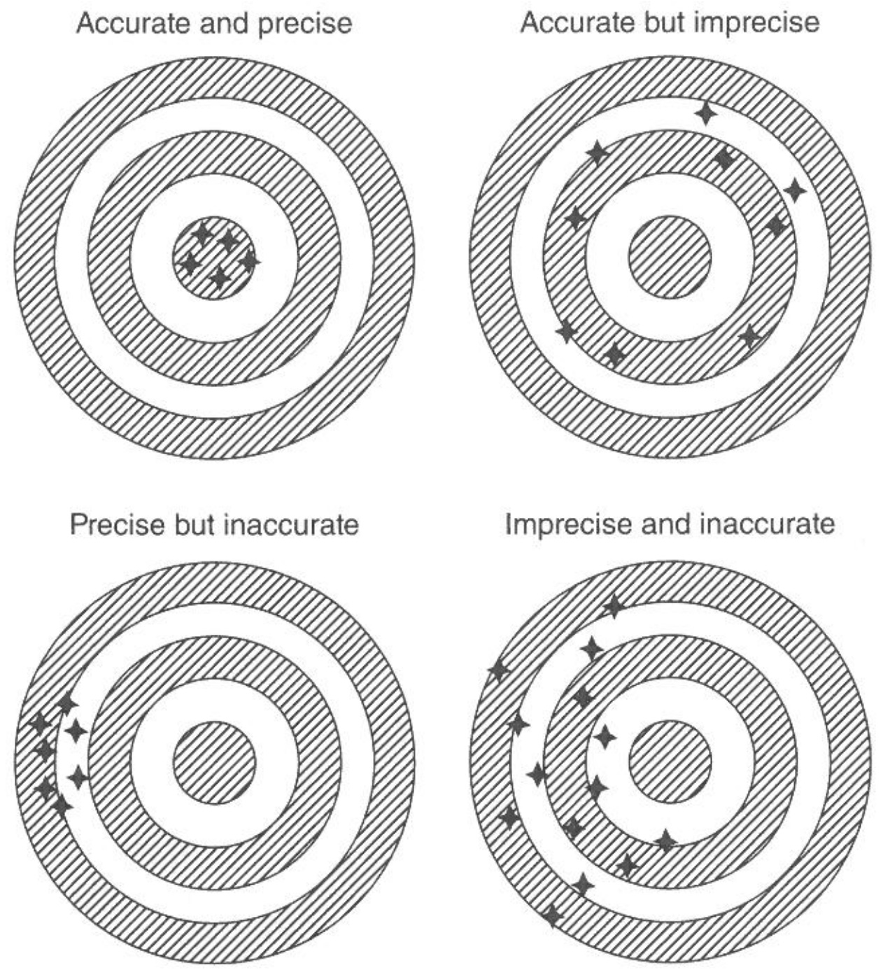
Precision and accuracy
Any measurement is carried out with a certain precision, which defines how much on average a measurements corresponds with the real value. Therefore, by definition, imprecise measurements add random error to a measurement. If the measure of the same entity is repeated many times, the real value may still be obtained but this can only be done if repeated measures are an option. For this reason, it is always best to maximise precision of a measurement.
Accuracy of a measurement expresses the fact that measurements are unbiased. In this context, bias or inaccuracy indicates whether there are any correlated deviations from the real value, for example because all measurements add a certain value to the measurements.
There are four possible combinations of high and low precision and inaccuracy, as shown in Figure 1.
Repeated measurements allow to estimate the precision and calibration with some ground truth allows to measure the accuracy. It should be noted, that there are technical replicates and biological replicates to estimate precision. Technical replicates are repeated measurements taken using the same sample and the same measurement technique. These replicates are used to assess the precision of the measurement technique, as variations in the results of the replicates can be used to estimate the uncertainty or error associated with the measurement. Biological replicates, on the other hand, are repeated measurements taken using different samples that are drawn from the same population. These replicates are used to assess the biological variability within a population, as variations in the results of the replicates can be used to estimate the natural variability or differences within the population. In general, technical replicates are used to assess the precision of a measurement technique, while biological replicates are used to assess the natural variability within a population.
Subsampling across sources of variation
If you conduct measurements across multiple entities that are a source of variation, a central question is how many samples to take from each entitities. These considerations should already play a role during the design of the experiments. Assume you want to measure the response of plants drought stress and you intend to do this by checking weather reports and sampling from farmers fields with low and high rain in a certain geographic region. The question is then whether it is better to measure many (e.g., 50) plants from two fields only, e.g., one with and one without drought stress, or whether it is better to sample fewer plants (e.g., 5) from a larger number of of fields (e.g., 10 with and 10 without drought stress). Sampling more plants within an entity such as a field will allow a better estimate of variation with in a field, but not between fields, whereas sampling a large number of fields will provide better estimates between but worse estimates within fields.
As a rule of thumb, the sampling should be designed in a way to capture the largest source and greatest amount of variation using prior information such as predictions of models or the results of preliminary studies. Another consideration is the expected level of differences within and between experimental units such as agricultural fields. In the above example, increasing the number of fields likely improves the estimate of variation and differences.
Sensitivity and specificity
Closely related and analagous to precision and accuracy are the concepts of sensitivity and specificity. Sensitivity is defined as the proportion of truly positive individuals that are recognized as positive by a test. In other words, an ELISA test which recognises 95% of plants that are truly infected with a certain pathogen as being infected has a sensitivity of 95%. Therefore sensitivity measures the proportion of true positive cases among all positive cases. The proportion of 100% - 95% = 5% is then the proportion of false negative individuals.
Specificity is defined as the proportion of truly negative individuals that are recognized as negative by a test. An ELISA test with a specificity of 80% indicates that 80% of plants that are not infected are recognised as such by a test. Therefore, specificity measures the proportion of true negative cases among all negative cases.
An ideal test has a very high sensitivity and specificity, but for technical reasons in the design of a test this is often difficult to achieve. For this reason, it is often necessary to predefince the accepted level of error and to design a test accordingly.
The confidence in the outcome of a test needs to be further put into the context of the prevalence of a condition such as a disease in a population. Prevalence is the frequency of a condition in a population. In order to account for the prevalence two measures were defined to measure the confidence in a test result.
The positive predictive value (PPV) of a test measures the the proportion of individuals that are classified by a test as positive and which are actually positives. It is defined as \[ % \begin{equation} \text{PPV} = \frac{\text{number of true positives}}{\text{number of true positives} + \text{number of false positives}} % \end{equation} \tag{1}\]
Equation Equation 1 can be modified by defining prevalence as the proportion of individuals that are actually positive at the time of the test which then leads to the following equation \[ % \begin{equation} \text{PPV} = \frac{\text{sensitivity} \times \text{prevalence}}{(\text{sensitivity} \times \text{prevalence}) + [(1-\text{specificity}) \times (1-\text{prevalence})]} % \end{equation} \tag{2}\]
The complementary measures can be defined as the negative predictive value (NPV) of a test, which measures the proportion of individuals that are classified by a test as negative and which are actually negatives: \[ % \begin{equation} \text{NPV} = \frac{\text{number of true negatives}}{\text{number of true negatives} + \text{number of false negatives}} % \end{equation} \tag{3}\]
Equation Equation 3 can be modified by defining prevalence as the proportion of individuals that are actually positive at the time of the test which then leads to the following equation \[ % \begin{equation} \text{NPV} = \frac{\text{specificity} \times (1-\text{prevalence})}{[\text{specificity} \times (1-\text{prevalence})] + [(1-\text{sensitivity}) \times (1-\text{prevalence})]} % \end{equation} \tag{4}\]
Importantly, both PPV and NPV strongly depend on the prevalence of the condition such as the frequency of pathogen infections in a population.
Intra-observer variability
Intraobserver variability arises if during the measurement of subjects that human observer or an instrument shows a (more or less) systematic change in measuring parameters, e.g., accuracy or precision. Such a change is also called observer drift, and it can be corrected by various measures. They include defining categories of measurements that are well defined and therefore easy to apply. In the case of human observers they would lead to a reduced tendency for a shift because the observer becomes tired. Another approach is to keep scoring cards or other reference material that allow an easy comparison with a reference. If it is known that a machine-based observation is available in addition to a human-based measurement, the machine-based method may be preferred if it can robustly implemented. On example is the measurement of degree of pathogen infection of plant leaves. Instead of scoring 5 grades of infection by humans, which may not be very precise and change during the analysis of many plant leaves, a machine based approach consisting of taking digital images and analysing them with image analysis software may reveal much more precise estimates with any bias.
Other measures to account for intra subject variability are repeated measurements, which allow to calculate a repeatibility score. For this, an observer repeats the measurements of multiple subjects and then calculates a correlation between the measurements.
Inter-observer variability
Inter-observer variability arise if different observers are used for measurements. In the context of agricultural science many such situations arise. For examples in multilocation field trials, different observers may be responsible for the observation of the same traits or if observations are to be taken over a long time span the observations may be carried out by different persons.
If different observers are responsible for different treatment groups or different locations of field trials, the variation among individuals may be confounded with the factors treatment or location that may cause differences and therefore lead to a bias in the results.
One solution to this problem is to distribute observers randomly over the experiment, they can be treated as blocks and included as such in the statistical analysis.
Machine-based, automated observations
One of the most powerful developments in avoiding both intra- and inter-observer variability as well as achieving highly precise and unbiased measurements is to use machine-based, automated observations.
This includes using laboratory robots for molecular assays, spectroscopic methods that often provide redundant information that is suitable for internal calibration as well as image based analysis methods for plant phenotyping using digital image analysis.
These approaches profoundly change the design and analysis of experiments because individual measures are much more precise and unbiased, but also can vastly increase the sample sizes compared to manual, human based measurements because they are cheaper. Therefore even small differences between subjects or small effect sizes in response to treatments can be measured with high precision.
For students of crop science therefore the ability and skill to develop new phenotyping technologies based on such technologies and machine-learning leads to better career options that traditional skills.
Decisions about how and what to measure
In manual measurements it may often be useful to define *discrete categories# that are expressed as scores, ranging from 1-10, for example, and who’s order expresses some quantitative variation. If the number of categories is small (‘no infection’, ‘mild infection’, ‘strong infection’ of a leaf with a pathogen), the repeatability for observations may be very high. On the other hand, the statistical power to identify subtle differences may be strongly limited.
Continous variables can be measured at different levels of resolution. One has to make a decision with respect to the level of resolution that is necessary to answer the scientific question at hand or which level of resolution can be achieved at a reasonable cost.
Taken together, the resolution of the measurement should correspond to the effect size. If the goal is to identify genotypes of a crop plant that carries a resistance gene against a pathogen, it may be sufficient to use only three criteria (as shown above) instead of using an elaborate phenotyping method to differentiate between 90% and 95% leaf area infected because in both cases the plant would be highly susceptible to a pathogen.
Biases in sampling and measurement
The above discussion of measurement shows that there are several biases inherent in sampling and measurements that need to be considered:
- observer bias (or experimenter bias, research bias) is any bias introduced by human involvment in the experiment
- affirmation bias expresses the scoring of an experiment based on ones bias with respect to the expected outcome
Some biases may occur conciously, others inconciously, but procedures such as blinding# in which the observer is blind to the treatment group or double blinding# in wich both the observer and the experimentator (or members of a treatment group) are blind to the treatment will help to avoid such biases.
- allocation bias refers to the bias of allocating certain groups to the treatment
- selection bias refers to the fact that a nonrandom set of individuals is selected for subsequent analysis
Floor effects# and ceiling effects# occur if individuals are selected either from the lower or higher end of the possible range of measurements.
Some useful guidelines for taking measurements
With respect to naming samples and measurements, follow a simple rule: explicit is better than implicit. In other words, give your samples and measures meaningful names (or abbreviations), insted of just naming them ‘A’, ‘B’, ‘C’ or the like. In any case write down the full meaning of measurements, i.e., create useful metadata.
- Back up your data more than once!
- Keep a laboratory book or an electronic lab journal.
- Do not overwork.
- Try to automate whereever you can or delegate your work to a machine or a software program.
- If you do automated data collection, check your collection setup regularly.
Summary
To be added
Key concepts
Further reading
- Lohr (2021) Sampling - Design and Analysis: A very comprehensive treatment of sampling. Chapter 2 is a good introduction into the topic.
Study questions
To be added
Exercises
Phenotyping the severity of an infection
Phenotyping by visual inspection is frequently used in field trials of crop plants. Frequently a so-called grade-scale is used in which quantitative phenotypes are translated into grades. The scoring card in Figure 2 is an example for this type of phenotyping. The disease severity is measured the the proportion of leaf area affected by the disease.
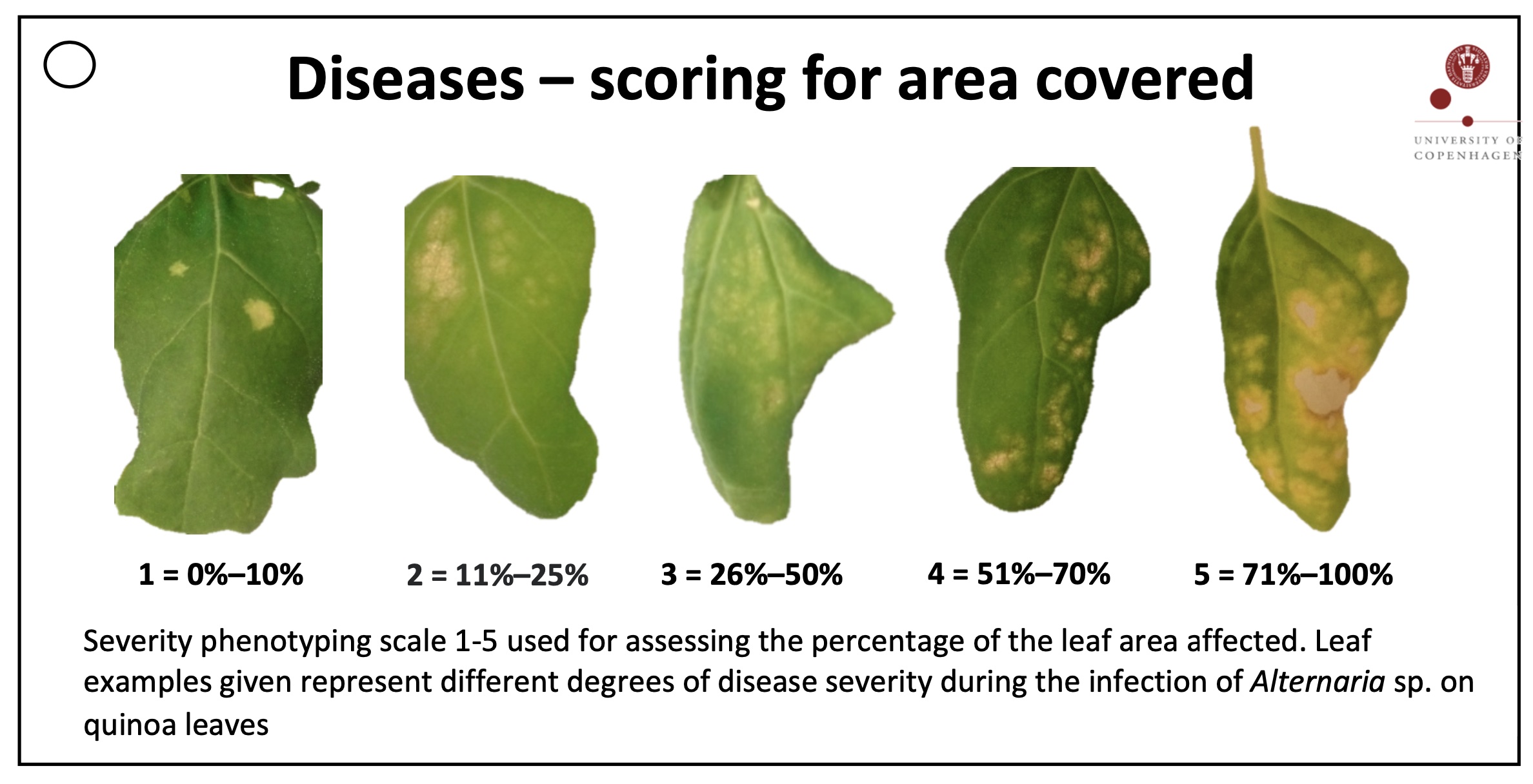
In this exercise, we create a dataset by phenotyping the leaves in Figure 3 using the phenotyping card in Figure 2. The leaves were inoculated under controlled conditions with the downy mildew pathogen Peronospora variabilis (Colque-Little et al. (2021)).
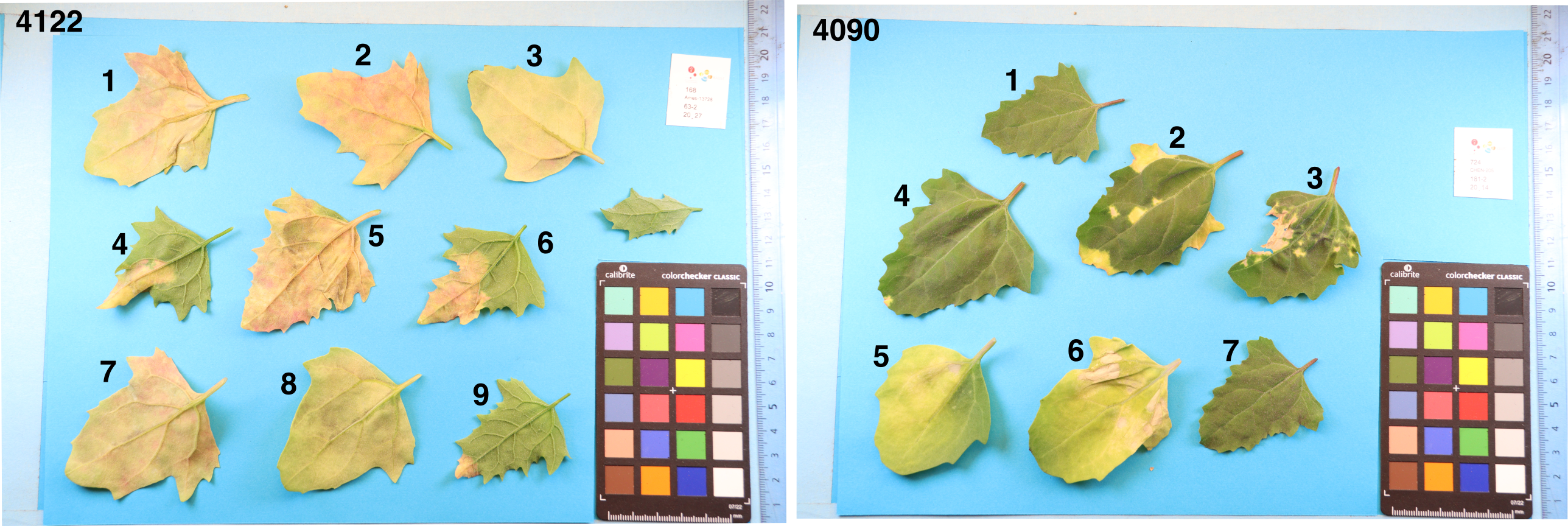
Please individually record the following data:
- Your matriculation number
- The plant number (number on top left, i.e., 4122 or 4090)
- The leaf number
- The degree of severity of each leaf based on the scale in Figure 2
Collect the data in a spreadsheet, merge the data and analyse them together with respect to intersubject variability and other factors