Scientific reasoning with probabilities
A motivating example
The application of probability theory is at the core of modern scientific investigations. We can demonstrate this fact with the following example.
Enzyme-linked immunosorbent assays (ELISA; Wikipedia) are widely used for the detection of viral and bacterial pathogens in plants. The assays consist of antibodies that recognize pathogen proteins and, upon recognition result in a color reaction that can be detected (Figure 1).

Frequently, assays are designed to recognize a multitude of pathogens. A positive color reaction suggests the presence of a pathogen in plant tissue. Such a test should answer the following questions:
- What is the probability that a positive ELISA test correctly identifies a pathogen?
- Does the ELISA test recognize all variants (strains or races) of a pathogen?
- How plausible is a positive test result if we know a priori that a pathogen is very rare?
These questions can be answered by applying probability theory to the test results.
We first begin with a formal definition of probability theory, and then derive Bayes’ Theorem, which is an important tool to answer applied questions in scientific research. In the end, we demonstrate a few fallacies in the context of probability theory.
Relationship between probability theory and statistics
Probability theory is derived from deductive logic, whereas statistics is derived from inductive logic. Both are tools for scientific inference.
Many decisions in life, science and politics are based on more or less conscious probabilistic arguments. However, misuse and abuse of probability and statistics is common, even in science (Figure 2). For this reason it is important to know the foundations of probability and statistical analysis.
An philosophical introduction into probability
We begin with conceptual ideas of probability. Analogous to the discussion on the scientific method we can differentiate two meanings of probability.
The first comprises objective or physical probability is the chance of an event occurring.
The second meaning is the subjective, personal or epistemic probability, which the degree of belief in a statement that is based on experience.
The objective probability of an event exists independently from the subjective probability, analogously to a natural phenomenon and statements about phenomena that we develop based on the scientific method.
These different meanings of probability can be demonstrated using the examples in Figure 3.
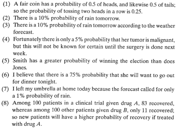
These eight statements can be interpreted differently, because they express different meanings of probability.
- The statement is deductive, apodictive and self-evidently true.
- This is an empirical statement without evidence.
- This is an empirical statement with a source of evidence, but no evidence itself.
- Here, the probability refers to knowledge but not the fact itself. The probability may change with additional knowledge.
- This is a statement about a relative probability, but the information is incomplete.
- This statement expresses a subjective estimate of probability, but no evidence is given.
- Here, probability is used as basis for decisions and actions. Its value is part of a cost/benefit analysis.
- This is an example of induction: Two singular observations are compared and a general conclusion is derived.
There are different aspects in the definition of probability:
- Events versus beliefs
- Repeatable versus single events
- Expression in exact numbers versus inexact beliefs
- A function of one argument (event) or two arguments (event and evidence)
- Should one combine or not combine old and new information?
- Effects of ignorance versus knowledge on probability statements
- Combination of theoretical and empirical aspects of probability
- Connection between deductive and inductive applications?
- Single theory of probability for all situations possible?
These aspects determine how we approach probabilistic reasoning.
Additionally, there are some fundamental requirements for probabilistic reasoning:
- Generality
- A good theory of probability should works for all cases and persons
- Impartiality
- A good theory of probability must be fair to all hypotheses
From these considerations one can derive eight general rules for a concept of probability (Gauch Jr, 2012):
- Explicit: Each statements needs to express its presuppositions and conclusions.
- Coherent / self consistent: It needs to follow the structure of deductive logical arguments.
- Practical: Experiments should be possible to validate statement about probability.
- Revisable: If new mathematical theories are data become available, the statements about probabilities should be revisable.
- Empirical: Conclusions must be dominated by evidence.
- Parsimonious: The number of axioms for statements about probability should be small.
- Human: Probabilistic reasoning must be ompatible with humaness and imperfection.
- Not perfectionistic: Statements about probability should be able to take care of experimental error.
A first definition of probability
For a more formal treatment of probability, we begin with the simple example of relative frequencies, which may serve as a first definition of probability.1
Consider a finite set of objects with different traits \(A\), \(B\), \(\ldots\). Define the relative frequency (\(\text{fr}()\)) of trait \(A\) as \[\begin{equation} \label{prob} \text{fr}(A)=\frac{\text{number of objects in the set with trait\ } A}{\text{total number of objects in the set}} \end{equation}\]
We define probability as a fraction of the finite set, i.e., the probability of \(A\) is then \(\text{fr}(A)\). The relative frequency of objects with a specific trait observed so far is then considered to be a predictor for the number of objects with the trait among a set of newly observed objects.
The statements require the acceptance of principle of a uniformity of nature (UN) (See the discussion on Hume’s problem in the class on scientific reasoning) such that the frequency of object with trait \(A\) in the original and in the new set are the same.
The above statement then has several properties:
- Relative frequencies are values \(\geq 0\)
- The relative frequency of objects with any trait is 1. In other words the total frequency of all traits in a set is 1
- For mutually exlusive traits \(A\) and \(B\), \(\text{fr}(A)\) or \(\text{fr}(b) = \text{fr}(A) + \text{fr}(B)\)
These properties are the basis of the concept of probability. From these, an axiomatic definition of probability can be derived as was done by the Russian mathematician Kolmogoroff in the 1930’s. For a recapitulation, an axiom is a statement that is accepted as self-evident truth of a domain and is then used to derive further further true statements in a deductive manner.
Kolmogoroff’s probability axioms are as follows:
- The probability of getting a particular outcome is expressed as value \(\ge 0\)
- The probability of getting any possible outcome is 1
- The probability of getting either of two mutually exclusive outcomes equals the sum of the probabilities of these outcomes.
These axioms can be explained with an example. We toss two coins and set the probability for each of the four outcomes to \(\frac{1}{4}\). Based on Kolmogoroff's axioms, we can conclude:
- The probability of getting two heads is \(1/4\)
- The probability of getting any outcome, namely two heads or two tails or else one heads and one tails, is 1.
- The probability of getting two heads, or else one heads and one tails is \(1/4+1/2=3/4\)
We can express these staments somewhat differently:
- Statement 1:
- The probability of an ideal fair coin landing heads is \(1/2\).
- Statement 2:
- The probability of an actual fair coin landing heads is nearly \(1/2\).
- Statement 3:
- The probability that my belief `The fair coin will land heads’ will be true is \(1/2\).
Then it is possible that these statements, which are derived from the three axioms, include favorable properties of a general and impartial probability theory.
- They reflect abstract entitities (Statement 1) and can be used for deductive statements
- They represent actual (empirical, observed) events (Statement 2) and allow inductive statements
- They enable the expression of personal beliefs (Statement 3) and quantify the degree of belief.
Therefore, the theory serves applications in daily life and scientific inference, as we have postulated above.
A formal definition of probability axioms
Using mathematical annotation, we develop a formal definition of probability axioms. Let us first give some formal definitions:
- Two sets \(A=\{1,2\}\) and \(B=\{2,3,4\}\)
- Union of two sets: \(A \cup B = \{1,2,3,4\}\)
- Intersection of two sets: \(A \cap B = \{2\}\)
- Subset: \(\{2\}\) of \(\{1,2\}\) but not of \(\{3,4\}\)
- Mutually exclusive sets: \(C=\{2\}\) and \(D=\{3,4\}\). Formally, mutual exclusivity is written as \(C\cap D=\emptyset\) (empty set)
- Complement sets: All possible outcomes form the set \(\Omega\). Let \(A\) be a subset of \(\Omega\). The complement \(\neg A\) of \(A\) consists of all outcomes in \(\Omega\) which are not in \(A\).
Using these definitions, we can express Kolmogoroff’s axioms in formal language. Let \(\Omega\) be a finite set of outcomes and \(A\) and \(B\) two subsets of \(\Omega\). \(P\) is then a probability measure if
- Axiom 1: \(0\leq P(A)\)
- Axiom 2: \(P(\Omega)=1\)
- Axiom 3: If \(A\cap B=\emptyset\), then \(P(A\cup B)=P(A)+P(B)\)
Formal probability theory has some advantages:
- Thoughts expressed in probability theory have a common structure and predictability.
- The thinking is public, therefore a common understanding is possible.
Both characteristics are essential components of the scientific method.
Conjunction
The intersection of two sets \(A \cap B\) is a conjunction. if \(A\) and \(B\) are logical statements, then the conjunction of both sets is true is \(A\) and \(B\) are true. Therefore, the conjunction is equivalent to a logical “and” operation.
If \(A\) and \(B\) are two Boolean sets of elements (Boolean sets are lists of true and false values with a relative frequency of both values), a conjunction is the frequency of items in a set in which both elements with traits \(A\) and \(B\) are true.
Consider the following example. Assume that we search for a genebank accession that is resistant against a certain plant pathogen. For this, we screen 100 accessions for disease symptoms after infecting them with the pathogen and obtain the following values (Table 1).
| No symptoms | Symptoms | Marginal | |
|---|---|---|---|
| Resistant | 4 | 1 | 5 |
| Susceptible | 5 | 90 | 95 |
| Marginal | 9 | 91 | 100 |
The conjunction of resistant accessions with no symptoms is then \(P(\text{No Symptom} \cap \text{Resistant}) = \frac{4}{100} = 0.04\).
Note that conjunctions are commutative, i.e., \(A \cap B = B \cap A\), which we will use later.
Conditional probability
A conditional probability is a probability that depends on a condition. For example, the probability of a hypothesis, \(H\), given the data, \(D\): \(\text{P(H|D)}\), is a conditional probability. Both \(H\) and \(D\) are subsets of outcomes, \(P(D)>0\).
Assume we have two events \(A\) and \(B\). Their joint probability is calculated as \(A \cap B\) is calculated by weighting the conditional probability of \(A\) given \(B\) by the marginal probability of \(B\). The marginal probability of \(B\) is just its probability. \[\begin{equation} \label{condcalc1} P(A \cap B)=P(A|B)P(B) \end{equation}\] When \(A\) and \(B\) are independent, \[\begin{equation} \label{condcalc2} P(A \cap B)=P(A)P(B) \end{equation}\] Dividing both sides of \(\eqref{condcalc1}\) by \(P(A)\) and assuming that \(P(B) \neq 0\), we obtain the definition of the condidtional probability of \(A\) given \(B\) is \[\begin{equation} \label{condcalc3} P(A|B)=\frac{P(A \cap B)}{P(B)} \end{equation}\]
We can express this in words: To evaluate the probability that \(A\) occurs in the light of information on \(B\), the probability that they occur together can be evaluated as \(A \cap B\), relative to the chance that \(B\) occurs at all, which is \(P(B)\).
The formal definition of conditional probability is then \[\begin{equation} \label{condprob} P(H|D)=\frac{P(H \cap D)}{P(D)} \end{equation}\]
Equation \(\eqref{condprob}\) has the following interpretation: Knowing that the actual outcome of an experiment is in \(D\), what is the probability that an outcome of \(H\) has happened?
It needs to be noted that a conditional probability is not commutative.
Therefore, \(P(H|D)=\frac{P(H \cap D)}{P(D)}\) has a different interpretation than \(P(D|H)=\frac{P(H \cap D)}{P(H)}\), the latter meaning ‘Knowing the probability of an hypothesis, what is the probability of the data given a hypothesis’.
The non-commutativity of conditional probability will be important in the derivation of Bayes’ theorem.
Let us demonstrate conditional probability with a few examples.
Example 1
Assume there are resistant and susceptible plants in your experiment. All plants are infected with a pathogen and symptoms examined. Resistant plants: 8 plants develop no symptoms and 2 plants do. Susceptible test: 1 plants develops no symptom and 13 do.
Unconditional probability of resistance in plants: \[\begin{equation} \frac{8 + 1}{10 + 14} = 0.375 \end{equation}\]
Conditional probability of resistance in resistant plants: \[\begin{equation} P(H|D)=\frac{P(H \cap D)}{P(D)} =\frac{8}{10} = 0.8 \end{equation}\]
Conditional probability of resistance in susceptible plants: \[\begin{equation} P(H|D)=\frac{P(H \cap D)}{P(D)} =\frac{1}{14} = 0.07 \end{equation}\]
Example 2
Assume that we search for a genebank accession of wheat that is resistant against a certain pathogen.
For this, we screen 100 accessions for disease symptoms after infecting them with the pathogen.
Our goal is to calculate the conditional probability of no symptoms given an accession is resistant (Table 2).
| No symptoms | Symptoms | Marginal | |
|---|---|---|---|
| Resistant | 4 | 1 | 5 |
| Susceptible | 5 | 90 | 95 |
| Marginal | 9 | 91 | 100 |
The unconditional probability that an accession without symptoms is resistant is then \(\frac{9}{100} = 0.09\)
The conditional probability of an accession is
- \(P(\text{No Symptom} \cap \text{Resistant}) = \frac{4}{100} = 0.04\)
- \(P(\text{Resistant}) = \frac{5}{100} = 0.05\)
Then we can derive:
\[\begin{equation} \label{probcond} P(\text{No Symptom} | \text{Resistant}) = \frac{P(\text{No Symptom} \cap \text{Resistant})}{P(\text{Resistant})} = \frac{0.04}{0.05} = 0.8 \end{equation}\]
Probability in action: Deduction of conclusions
Let us demonstrate probability theory in action by the deduction of some conclusions.
- Conclusion 1: \(P(\neg A)=1-P(A)\)
Proof: \(A\) and \(\neg A\) are mutually exclusive (\(A\cap \neg A=\emptyset\)) and \(A\cup \neg A=\Omega\). \[\begin{equation} \label{prob1} 1=P(\Omega)=P(A)+P(\neg A) \end{equation}\]
- Conclusion 2: \(P(B)=P(B|A)P(A)+P(B|\neg A)P(\neg A)\)
Proof: \(B=\underbrace{(A\cap B)}_:=C\cup\underbrace{(\neg A\cap B)}_:=D\). \(C\) and \(D\) are mutually exclusive, so \[\begin{equation} \label{prob2} P(B)=P(C)+P(D)=P(B|A)P(A)+P(B|\neg A)P(\neg A), \end{equation}\]
since \(P(C)=P(A\cap B)=P(B\cap A)=P(B|A)P(A)\) by the definition of conditional probability and analogously \(P(D)=P(B|\neg A)P(\neg A)\)
All theorems/techniques in probability are deducted from the probability axioms in this way.
Bayes’ Theorem
Bayes’ theorem dates back to the work of Reverend Thomas Bayes (1702 - 1761; Wikipedia). The theorem describes the degree of confidence given prior evidence.
The simple form of Bayes’ Theorem is defined as2 \[\begin{equation} \label{bayestheorem} P(H|D) \propto P(D|H) \times P(H) \end{equation}\] or, in simpler terms:
Posterior probability \(\propto\) Likelihood \(\times\) Prior probability
In contrast to the terms prior probability and posterior probability, we define the term likelihood as How likely is it that the observed data are produced under a given hypothesis, but keep in mind that the likelihood is also a probability.
The complete form of Bayes’ Theorem is
\[\begin{equation} \label{bayestheorem2} P(H|D)=\frac{P(D|H)P(H)}{P(D)}=\frac{P(D|H)P(H)}{P(D|H)P(H)+P(D|\neg H)P(\neg H)} \end{equation}\]
In the following, we derive a proof of Bayes’ Theorem.
Bayes’ Theorem: \[\begin{equation} P(H|D)=\frac{P(D|H) \times P(H)}{P(D)} \end{equation}\]
Rearrange the definition of conditional probability: \[\begin{equation} P(H \cap D) = P(H|D) \times P(D) \end{equation}\] Second application with \(H\) and \(D\) reversed: \[\begin{equation} P(D \cap H) = P(D|H) \times P(H) \end{equation}\] \(H \cap D\) and \(D \cap H\) are same set, so \[\begin{equation} P(H \cap D) = P(D \cap H) \end{equation}\] Equate the formulas to obtain \[\begin{equation} P(H|D) \times P(D)=P(D|H)\times P(H) \end{equation}\]
Ignore normalizing constant, \(P(D)\) and substitute proportionality for equality, we get Bayes’ theorem in simple form. Use Conclusion 2 to get the complete form.
The terms in Bayes’ theorem have the following meaning:
\[\begin{equation}P(H|D) \propto P(D|H) \times P(H)\end{equation}\]
- \(P(H)\): Prior probability or just prior
- \(P(D|H)\): Likelihood. Data’s impact on the probabilities of hypotheses, e.g. the likelihood that the hypothesis \(H\) generates the observed data \(D\).
- \(P(H|D)\): Posterior probability or posterior
Overall, Bayes theorem can be summarized as follows
Bayes’ theorem solves the inverse or inductive problem of calculating the probability of a hypothesis given some data \(P(H|D)\) from the probability of some data given a hypothesis \((D|H)\)
One advantage is that Bayes’ theorem can be expanded to make statements about competing, mutually exclusive hypotheses.
The formula for two hypotheses (\(H_2=\neg H_1\)) is then
\[\begin{equation} \label{bayestwo} P(H_1|D) = \frac{P(D|H_1)\times P(H_1)}{(P(D|H_1)\times P(H_1))+(P(D|H_2)\times P(H_2))} \end{equation}\] The formula for multiple hypotheses is then \[\begin{equation} \label{bayesmultiple} P(H_1|D) = \frac{P(D|H_1)\times P(H_1)}{\sum_{i=1}^n(P(D|H_i)\times P(H_i))} \end{equation}\] The ratio form compares hypotheses in forms of ratios or odds \[\begin{equation} \label{bayesratio} \frac{P(H_1|D)}{P(H_2|D)} = \frac{P(D|H_1)}{P(D|H_2)} \times \frac{P(H_1)}{P(H_2)} \end{equation}\]
Define
- \(H:=\text{selected individual is from Subpopulation 1}\)
- \(D:=\text{selected individual is heterozygous}\)
We already know
- \(P(H)=P(\neg H)=0.5\), since both subpopulations are equal in size
- \(P(D|H)\) is the probability that, if we pick from Subpopulation 1, we pick a heterozygous individual, which is the frequency of heterozygotes in SP1, hence \(P(D|H)=0.5\). Analogously \(P(D|\neg H)=0.25\), since this is the the probability that, if we pick from Subpopulation 2, we pick a heterozygous individual
We want to compute \(P(H|D)\). Using Bayes’ Theorem,
\[\begin{equation} P(H|D)=\frac{P(D|H)P(H)}{P(D|H)P(H)+P(D|\neg H)P(\neg H)}\\ =\frac{0.5\cdot 0.5}{0.5\cdot 0.5+0.25\cdot 0.5} \\ =\frac{2}{3} \end{equation}\]
This application is a demonstration of the famous Monty Hall problem, which was popularized in an American TV show (Wikipedia).
Common fallacies in probability theory
Although the probability rests on few foundations only, there are multiple opportunities for errors. These errors can be broadly classified as ignored priors and ignored conditions.
Ignored prior or neglect of probability
This fallacy reflects a bias in a judgement or decision under uncertainty that is based on probabilistic reasoning, which does not consider probabilistic information. It applies in particular to events that are very rare or show extremely unlikely outcomes (e.g., terrorist attacks, winning big in a lottery).
With this error, we demonstrate the application of probability to the testing of diseases.
Assume that you want to use an ELISA test for a rare disease that occurs by chance in 1 in every 100,000 trees (e.g., mango, Mangifera indica).
The test is fairly reliable: if a tree has the disease it will correctly say so with probability 0.95. If a tree does not have the disease, the test will wrongly say it does with probability 0.005.
If the test says your tree will suffer from the disease, what is the probability that this is a correct diagnosis?
A first assumption would assume to that it is 0.95, but this assumption is incorrect.
The solution can be concluded as follows.
- Probability that your tree has the disease, \(P(D)=0.00001\)
- Probability that your tree does not have the disease, \(P(\neg D)=0.99999\)
- Probability of positive test when the tree has the disease, \(P(T|D)=0.95\)
- Probability of positive test when the tree is healthy, \(P(T|\neg D)=0.005\)
Probability of disease given positive test result is then
\[\begin{eqnarray} \label{probeexercise} P(D|T) & = & \frac{P(T|D) \times P(D)}{P(T|D)\times P(D) + P(T|\neg D)\times P(\neg D)} \nonumber \\ & = & \frac{0.95 \times 0.00001}{(0.95 \times 0.00001) + (0.005 \times 0.99999)} \nonumber \\ & \approx & 0.002 \nonumber \end{eqnarray}\]
Keep in mind: \(P(T\|D) \neq P(D\|T)\)!
Ignored condition or conjunction fallacy
If a conjunction (joint occurrence) of two events is considered more likely than either one of the events on their own.
An example of the ignored condition is shown in the application of resistance genes.
A plant may be resistant to two pathogens \(P_1\) and \(P_2\): \(P(P_1 \text{resistance})=P(P_2 \text{resistance})=0.5\)
Four possible combinations of resistances are: None, \(P_1(=(P_1,\neg P_2))\), \(P_2(=(P_2,\neg P_1))\), \((P_1,P_2)\).
We assume that resistance to each pathogen is independent from the other resistance: \(P(P_1,P_2)=0.5^2=0.25=P(P_1)=P(P_2)=P(\mbox{none})\)
Question 1: What is the probability a plant has both resistances?
The answer is \(Prob = 1/4\).
Question 2: A plant has one of the two resistances. What is the probability that it also has the other resistance? Is it again \(\frac{1}{4}\)? Is it \(\frac{1}{2}\)?
Answer: No resistance is not possible; hence: \((P_1,P_2)\), \(P_1\), \(P_2\) \(\rightarrow Prob=1/3\)
Formal derivation using conditional probability
- \(X\): There is at least one resistance
- \(Y\): \(P_1P_2\) resistance
- \(P(X) = 3/4\) (3 of 4 combinations have a resistance)
- \(P(X \cap Y) = 1/4\) (only 1 of 4 has both resistances)
Hence: \(P(Y|X) = P(X \cap Y)/P(X) = (1/4)/(3/4)=1/3\)
Summary
- The concept of probability is useful for deduction and induction as part of scientific reasoning
- Formal definition of probability theory rests on few axioms
- Theorems can be derived from the axioms
- Bayes’ Theorem measures confidence in hypothesis given data
- Fallacies in probability theory: Incorrect use of prior probabilities; neglect of prior information
Key concepts
Further reading
Study questions
- Could Bayes’ theorem be useful for inductive procedures? How and why?
- A test for skabies. Skabies is a contageous skin disease that is caused by mites. Assume a test that predicts 98% correctly to healthy people that they are free of skabies, and 98% correctly to sick people that they have skabies. We assume that 1 in 1,000 inhabitants in our city have skabies. The test is positive for you.
- What is the probability that you have skabies given the positive test?
- What is the probability if you use a flat prior (e.g., an equal probability of all possible hyptheses), i.e. a probability of skabies = 0.5?
- Find examples for the errors Ignored prior and Ignored condition surrounding Bayes’ theorem.
In class exercises
Expectation of an election
An election is coming up and a pollster claims that candidate A has a 0.9 probability of winning. How do you interpret this probability?
- If we observe the election over and over, candidate A will win roughtly 90% of the time.
- Candidate A is much more likely to win than to lose.
- The pollster’s calculation is wrong. Candidate A will weither win or lose, thus their probability of winning can only be 0 or 1.
Probability of an event
Which of the expressions below correspond to the statement: /the probability of rain on Monday/?
- Pr(rain)
- Pr(rain|Monday)
- Pr(Monday|rain)
- Pr(rain, Monday)/Pr(Monday)