Models and model selection in science
Motivation
Models are a formal description of our knowledge and a necessary tool for scientific research. They play an important part in the scientific endeavor, and are in particular used in statistics where different models are investigated and compared. For example, models are frequently used to calculate the probability of the data, given a hypothesis (that is based on a model) for Bayesian analysis.
For this reason, it is important as a scientist to think in models and hypotheses, and not only in terms of data and descriptive analyses.
Nevertheless, a scientist also needs to consider the type of data that are produced in a scientific inquiry because they determine the set of analysis tools and methods, as well as the type of models to be used for the analysis.
Important dimensions to consider in models are
- Time scales
- Ability to replicate an experiment
- Ability to control the aspects of an experiment
Learning goals
Understand the concept of strong inference and how it can be used to systematically develop and test scientific hypotheses by devising alternative explanations and crucial experiments.
Learn how to develop and select scientific models by balancing complexity and explanatory power through the principle of parsimony, considering factors like predictive accuracy and testability.
Distinguish between different types of models, hypotheses, and theories, and recognize how they interact to help scientists understand and predict complex phenomena.
Develop skills in identifying and separating signal from noise in scientific data, understanding how statistical techniques can help in making more accurate scientific inferences and predictions.
Strong inference
We begin with a discussion of the concept of strong inference, which is based on the formulation of good, testable hypotheses.
Platt (1964) emphasised the importance of the inductive-deductive method/Baconian induction in science. He summarized this methods as strong inference about a phenomenon:
- Devising alternative hypotheses.
- Devising a crucial experiment (or several of them) with alternative possible outcomes. Each of the outcomes will exclude one or more of the other hypotheses.
- Carrying out the experiment to get clean results.
- Recycling the procedure, making sequential hypotheses to refine the possibilities that remain.
By recycling the procedure, Platt describes this process as tree climbing where the outcome of a given experiment describes the next experiment and the direction of the climb within a tree. He calls this approach to science as strong inference, because it leads to a robust body of knowledge. One assumption of this view is that the outcomes of experiments are unambiguous and that no statistics is needed.
Platt stressed that in such experiments, any test can not be only against a simple hypothesis, but against multiple hypotheses. In this, he extends the philosophy of Karl Popper. Another conclusion of Platt is that in scientific fields where strong inference is possible, scientific progress is faster.
Note that strong inference leads in every turn to the experimental testing of parts of the complete theory (Step 3) as well as further logical analysis and expansion (Step 1) of a theory.
Platt argues that
- strong inference is responsible for most rapid development in any field of science.
- work spent on theory-building and experimental design not linked to one of the steps is not well-invested.
- strong inference uses the minimal number of steps to come to scientific progress.
- thinking about several hypotheses forces to really search for evidence for each hypothesis (and not to ignore evidence not matching your pet hypothesis).
What are the outlines of these considerations for practical scientific aspect? First, it may be worthwile to consider and test multiple hypotheses from the beginning of a scientific study. Second, focus your resources on a single or few well-designed and powerful experiments that have the greatest power to differentiate between these hypotheses. Third, keep a diversity of methods in mind that allow to validate hypotheses in subsequent experiments.
Theories, hypotheses and models
Formal definitions
It is necessary to differentiate between the concepts of theory, hypothesis and model.
A theory was defined in Webster’s dictionary as ‘considerable evidence in support of a general principle, explain the operation of certain phenomena’. Theories do not necessarily have to be quantitative, for example the Theory of Evolution by Charles Darwin is based on three (non-quantitative) principles. These principles of Darwin’s theory are:
- Variation between individuals;
- Inheritance of traits
- Differential reproductive success.
Any system in which these three principles are valid will show evolutionary progress.
A hypothesis according to Webster’s dictionary ‘implies an inadequacy of support of an explanation that is tentatively inferred, often as a basis for further experimententation’. A good scientific hypothesis is a statement that has the property that it can be falsified in the Popperian sense.
Finally, the term model originated from the latin word modus, which means ‘the way things are done’. According to Webster’s, a model is a ‘stylized or formalized representation or a generalized description used in analyzing or explaining something’. In other words, a model is a formal description of our knowledge about a phenomenon. It may be a simplified description of reality. A good model should allow predictions, which resemble hypotheses that can be falsified. Models may be expressed completely or partly in mathematical language, but they do not have to be.
For example, in population genetics, famous and useful models are the Hardy-Weinberg equilibrium for describing frequencies of genotypes in populations under random mating, or the Fisher-Wright model for describing change in allele frequency between generations.
The relationship between a hypothesis and models can be complicated because there can be different models for the same hypothesis. According to Popper, however, only a single hypothesis or model are always tested against a null hypothesis. If there are several models of a hypothesis, each model is falsified separately against the null hypothesis. Other philosophers of science like Platt or Lakatos postulate that the simultaneous falsification of hypotheses is possible.
The relationship between models and hypotheses can be represented by the following example.
- Theory:
- Nitrogen is required for plant growth because it is an essential component of proteins.
- Hypothesis:
- More nitrogen applied during plant growth leads to a higher yield.
- Null hypothesis:
- There is no effect of nitrogen fertilization on plant growth.
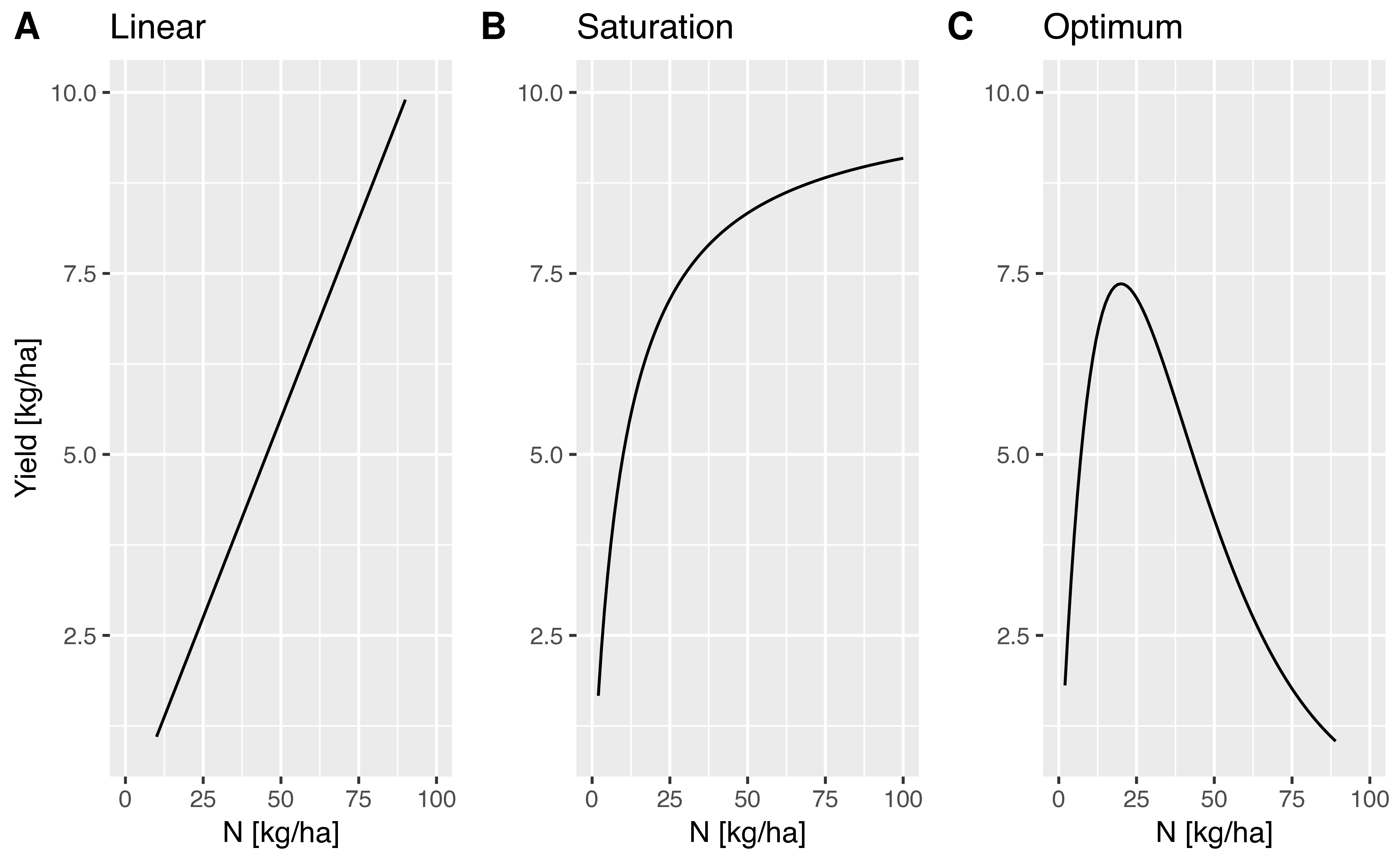
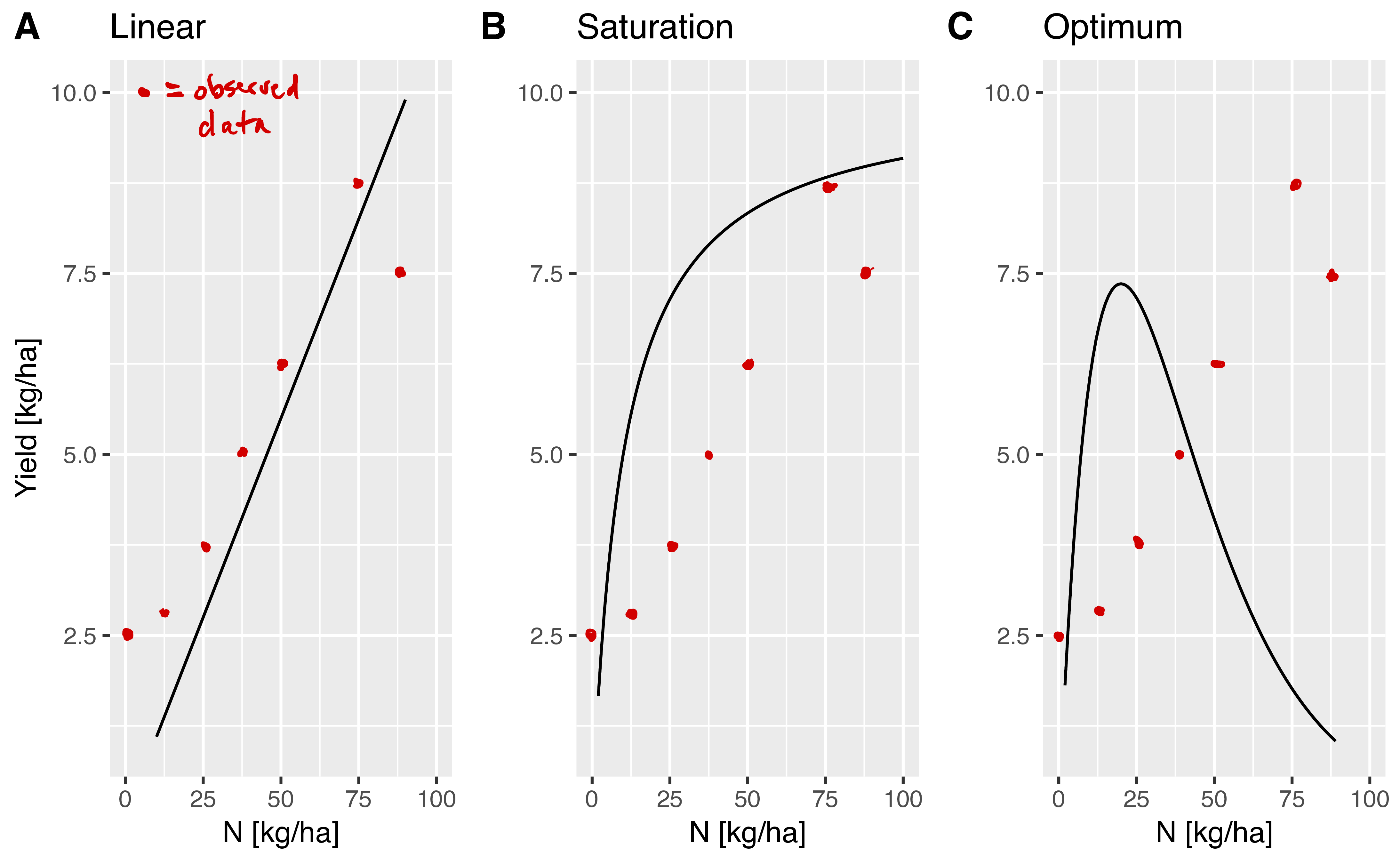
The hypothesis can be separated into different models that specify the hypothesis in greater detail. The models can be expressed mathematically.
- Model 1:
- Yield increases linear with the amount of nitrogen applied: \[\begin{equation} \label{linear} Y = aF \end{equation}\] where \(Y\) is yield, \(a\) is a constant and \(F\) is the amount of fertilizer.
- Model 2:
- Yield increase shows a saturation curve with increasing nitrogen application: \[\begin{equation} \label{saturation} Y = \frac{aF}{1+bF} \end{equation}\] where in addition to the above parameters, \(b\) is a second constant.
- Model 3:
- There is an optimal yield level with a certain amount of nitrogen applied. \[\begin{equation} \label{optimum} Y = aFe^{-bF} \end{equation}\]
The differences in the models is shown in Figure Figure 1.
Models have three components:
- Variables:
- They are changeable in the context of the model. Models have independent and dependent variables.
- Parameters:
- They are fixed in the model and can be estimated by fitting data to a model, e.g., by least square regression.
- Relationships:
- Variables and parameters have a relationship within a model that are described by mathematical, logical or other terms.
The models have several parameters, which in our example are \(a\) and \(b\). These parameters can be estimated with appropriate procedures.
Types of models
Models can be classified into different types that have frequently different uses.
- Deterministic versus stochastic models
- Scientific versus statistical models
- Static versus dynamic models:
- Quantitative versus qualitative models
Each type of model has different advantages and disadvantages and is used for various contexts, but we will not further discuss these models in detail.
Example of using a model and a hypothesis
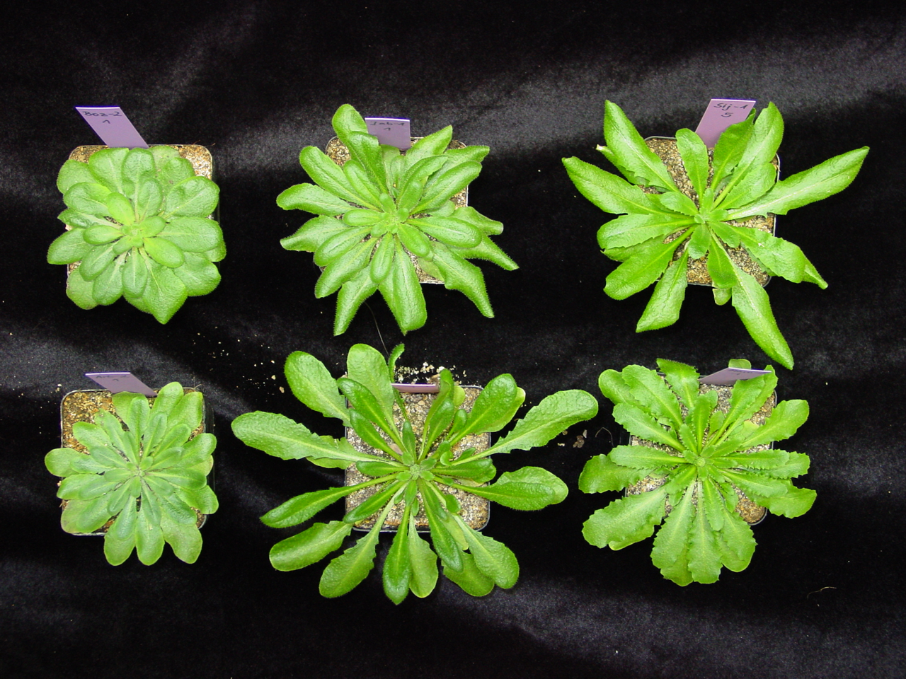
As mentioned before, the relationship between hypothesis and models is not so clear. Let us assume we want to investigate the causes of phenotypic diversity in a collection of the model plant Arabidopsis thaliana lines that were collected throughout the species range and represent different genotypes (Figure 2). These plants were cultivated under the same conditions in the greenhouse, therefore observed differences are most likely the result of genetic differences between the plants.
Assume that we are now interested in studying which processes generated the diversity. Based on prior knowledge about population genetics, one can propose two hypotheses:
- The phenotypic variation originated by genetic drift through the random fixation of mutations or
- by adaptation to the local environment by the fixation of adaptive mutations through natural selection.
The hypotheses can be expressed more formally:
- Question:
- Which processes shape patterns of genetic variation?
Possible hypotheses are:
- \(H_0\): Genetic drift (random evolution)
- \(H_1\): Natural selection (local adaptation)
We know, however, that there is not only one type of natural selection, but different types of selection, such as purifying selection (removal of disadvantageous mutations), positive selection (fixation of a single advantageous mutation) and balancing selection (maintenance of multiple advantageous mutations). Therefore, a single model of selection seems too simplistic and we should formulate models for the different types of selection and use one or all of these models to test against the null hypothesis:
- Question:
- Which processes shape patterns of genetic variation?
\(H_0\): Genetic drift (random evolution)
\(H_1\): Natural selection
- Model 1: Positive selection - Fixation of an advantageous mutation
- Model 2: Purifying selection - Removal of a deleterious (disadvantageous) mutation
- Model 3: Balancing selection - Maintenance of multiple advantageous mutations at intermediate frequencies
One has to make a decision which model of selection to take for the \(H_1\) that is tested against \(H_0\), because the three models are expected to produce different patterns of genetic and phenotypic variation in a population. Another fundamental problem is that phenotypic variation can be the consequence of the joint and simultaneous action of genetic drift and natural selection. Therefore, we need to write:
- \(H_0\): Genetic drift (random evolution)
- \(H_1\): Natural selection
- \(H_2\): Genetic drift and natural selection
This shows that the full range of models requires the comparison of multiple hypotheses. It is possible to test only against the null hypothesis of random evolution and ignore any other models or explanations like natural selection, or a combination of random evolution and natural selection. Such a focus on falsification in the sense of Karl Popper is a proper scientific approach, but our ability to learn something from the data is limited and unsactisfactory. A better approach is to formulate explicit models for each of the hypotheses that make predictions about the expected data and then compare observed data to model predictions, and select the best-fitting model given the data.
A nice but complex demonstration of the application of this concept in the context of model formulation and selection for natural variation of Arabidopsis thaliana is described by Huber et al. (2014).
Models and hypothesis in the context of population genetics
We consider another example from population genetics theory. Assume a species in which male and female gametes mate randomly to form the offspring. The biological process is also called random union of gametes.
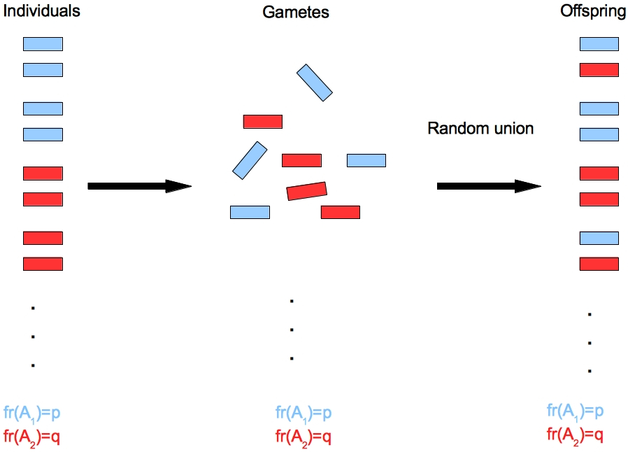
From a biological model of random union a hypothesis can be derived, which predicts the frequency of genotypies from individual allele frequencies according to the Hardy-Weinberg model (Wikipedia).
The observed allele frequencies are
| Allele type: | \(A_1\) | \(A_2\) |
| Frequency: | \(p\) | \(q\) |
and the predicted genotype frequencies based on observed allele frequencies are then
| Genotype: | \(A_1A_1\) | \(A_1A_2\) | \(A_2A_2\) |
| Hardy-Weinberg frequency: | \(p^2\) | \(2pq\) | \(q^2\) |
This model makes many assumptions for mathematical convenience. They include an infinite population size and random mating. We also assume that this model describes the allele and genotype frequencies at a biallelic locus in a very large diploid plant population with no selection and mutation.
From the model following hypotheses can be generated:
- Hypothesis 1:
- After only one generation of random mating, Hardy Weinberg frequencies for genotypes are achieved.
It is possible to develop a second model, which leads to a second hypothesis. The second model makes the same assumptions, but in addition male and female individuals are differentiated and random mating is allowed only between male and female individuals (in the previous model, individuals can have both sexes).
The second hypothesis is then
- Hypothesis 2:
- After one generation of random mating, genotype frequencies are
| Genotype: | \(A_1A_1\) | \(A_1A_2\) | \(A_2A_2\) |
| HW frequency: | \(p_mp_f\) | \(p_mq_f+q_mp_f\) | \(q_mq_f\) |
where \(p_f\), \(q_f\) are the allele frequencies of \(A_1\), \(A_2\) in the female population and \(p_m\), \(q_m\) the \(A_1\), \(A_2\) frequencies in the male population.
The next step is then to design an experiment that distinguishes between both models and the resulting hypotheses:
Hypothesis 1 predicts a frequency of \(2pq=\frac{1}{2}\) of heterozygotes in the \(F_1\) generation, Hypothesis 2 predicts a frequency of 1. The observed data can be compared with the expected outcome and the hypothesis that fits better to the data can be selected.
Testing hypotheses by taking samples from a population
Hypotheses making general predictions (e.g., all plants have DNA, all humans are sentient, smoking causes cancer) can be falsified directly by an experiment which finds one counterexample (for non-causal hypotheses, it also suffices to find one counterexample in the population).
For other hypotheses, looking only at a sample of cases will not allow to falsify directly. However, the sample allows to gather evidence for or against a hypothesis, particularly in comparison to other hypotheses. To measure the probability that a hypothesis is true compared to other hypotheses, a statistical framework has to be used.
As an example for the application of Bayesian statistics, the model described above will be investigated to differentiate between hypotheses.
Going back to our experiment, we may be not looking at the complete, very large \(F_1\) population, but only at a sample of \(10\) individuals. Let us assume that all indiviuals in the sample are heterozygous. Such a sample is possible under both hypotheses, but seems more likely for the second hypothesis.
To compare the posterior probability of both hypotheses given the sample, we can use Bayes’ theorem in ratio form: \[\begin{equation} \label{bratio} \frac{P(H_1|D)}{P(H_2|D)}=\frac{P(D|H_1)P(H_1)}{P(D|H_2)P(H_2)}. \end{equation}\]
We do not have any preference for any hypothesis before the experiment, so we set a uniform prior \(P(H_1)=P(H_2)=0.5\), which makes each of the two hypotheses equally likely. By inserting these values into Equation \(\eqref{bratio}\), one obtains \[\begin{equation} \label{bratio2} \frac{P(H_1|D)}{P(H_2|D)}=\frac{P(D|H_1)0.5}{P(D|H_2)0.5}=\frac{P(D|H_1)}{P(D|H_2)} \end{equation}\]
The likelihood of \(P(D|H_1)\) is the (binomial) probability of picking 10 heterozygous individuals \(P(D|H_1)=(\frac{1}{2})^{10}\), the likelihood \(P(D|H_2)\) is 1.
The ratio of the posterior probability is then \[\begin{equation} \label{bratio3} \frac{P(H_1|D)}{P(H_2|D)}=\frac{1}{2^{10}}=\frac{1}{1024} \end{equation}\]
Given the outcome of the experiment, Hypothesis 2 has a 1024 times higher posterior probability given the data Hypothesis 1. We now have to decide whether this difference in posterior probabilities makes us accept Hypothesis 2. For this hype of hypothesis testing, Kass, Robert E and Raftery, Adrian E (n.d.) have developed a scale for interpretation using the so-called Bayes Factor, which is essentially the ratio of the posterior probability of two hypotheses. The Bayes factor is defined as the \(log_{10}\) of the ratio of posterior probabilites, which in our case is 3.01. According to their scale a factor \(>2\) is “decisive” for one hypothesis over the other, and for this reason, we accept Hypothesis 2. It should be noted that instead of a Bayesian approach, the hypotheses could also be compared by analysing the sample in a frequentist approach, but then the hypotheses would have to be analysed separately.
Model selection
Frequently, different models can be developed for a given scientific question or problem, which leads to the question of which model should be selected as the one that best represents the data (and, by implication, reality).
Choosing the best theory
Theory selection is a more general term for model selection. It should address the question: What is a model good for? Therefore, we also need to ask: Which type of model should we use to study a scientific problem? And also the question: How complex should a model be?
Which model should be used?
Multiple types of models can be developed to describe the same biological phenomenon.
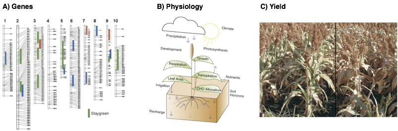
Example: Which model best describes the transition to flowering in plants? It is a very important trait for both plant breeding and cultivation, and an understanding of the factors that influence the transition to flowering has practical applications. Figure 4 shows different types of models that describe the regulation of flowering in plants.
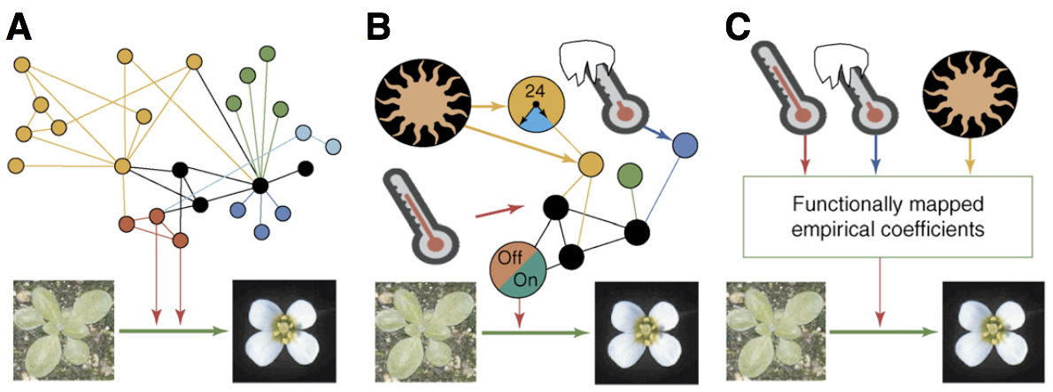
The first model shows a complete network of regulatory genes, but no environmental parameters. It has many components (genes) and can be used to investigate causal relationships and molecular interactions between genes to understand the molecular processes leading to flowering. The second model contains a few key genes and some environmental parameters such as day length, temperature, light exposure that have the biggest effect on flowering time and can be used to describe the interaction between environmental effects and selected genes in sufficient detail. The third model is an empirical model which contains only environmental parameters and derives some coefficients that can be used to predict the transition. Since no causal relationships are model, the process of transition to flowering is unknown and it is therefore a black box model
These models have different applications:
- Explain causal relationships among flowering genes and provide avenues for a genetic manipulation of flowering time.
- If the goal is to create photoperiod insensitive plants: Find the combination of environmental parameters and genes for achieving this goal.
- Breeding for climate change: make a predictive model to model the relationship between environmental parameters and yield, and use this information in plant breeding.
How many parameters should be included in a model?
Models have different levels of complexity, and the question arises, how many parameters should be included in a model, and what types of data should be used (Figure 5).
The question is whether some parameters are more important than others.
In the selection of models (also called theory choice) several aspects are important.
First, both data and models are important!
Additional criteria for selecting a model are the following principles:
- Parsimony:
- How complex does not model have to be?
- Predictive accuracy:
- How good are the predictions?
- Explanatory power:
- How well can the model explain results?
- Testability:
- Can the model be tested?
Further questions are:
- Is it possible to generate new insights and knowledge?
- Is it coherent with other scientific and philosophical theories?
- Can the results be repeated?
The parsimony principle
Definition and properties
One approach to select among models is to apply the parsimony principle, or Occam’s razor, which can be stated as:
Among theories that fit the data, choose the simpler one – William of Ockham (c. 1288- c.1348)

The principle of parsimony emphasizes that no insight is possible without simplification, as reducing complexity allows for a clearer understanding of essential concepts.
Parsimony encourages focusing on the most important aspects of a problem or system—identifying key variables or processes that drive the outcomes of interest.
This focus improves accuracy by removing unnecessary noise and reducing the risk of overfitting models or overcomplicating analyses that may reduce statistical power of an experiment.
The parsimony principle distinguishes between preferring a simpler model, which seeks an effective balance between simplicity and explanatory power, and preferring a simple model, which risks oversimplification at the cost of losing critical details.
In scientific and practical applications, the goal is to achieve the greatest insight with the fewest assumptions while retaining sufficient accuracy and relevance.
History of the principle of parsimony
The history of the parsimony principle can be traced back to ancient Greece, where early philosophers laid its foundations.
Plato taught the existence of ideal forms or “ideas” and their imperfect manifestations in the real world. Aristotle embraced the idea of parsimony as a key element of reasoning, distinguishing himself from his teacher Plato. Aristotle’s preference for focusing on tangible, observable realities was inherently more parsimonious than Plato’s metaphysical abstractions. Simplifying the world by discarding Plato’s notion of ideal forms marked an early application of parsimony.
In the medieval period, philosophers expanded on the principle of parsimony. Robert Grosseteste, the influential scholar at Oxford, and Thomas Aquinas in Paris articulated its importance in their reasoning, while William of Ockham provided one of its most enduring formulations, described above. Ockham famously argued that “entities should not be multiplied beyond necessity,” a principle now known as Ockham’s Razor, which emphasizes that simplicity should prevail unless complexity can be empirically justified. While Grosseteste focused on an ontological definition—suggesting that nature itself is inherently simple—Ockham leaned toward an epistemological definition, encouraging simplicity in the formulation of theories.
Several centuries later, the Copernican Revolution became a landmark example of the parsimony principle. In contrast to the geocentric model of planetary motion, which required complex epicycles to explain observations, Nicolaus Copernicus preferred the heliocentric model due to its simplicity and elegance. Although empirical evidence like stellar parallax (that were observed by Friedrich Bessel in 1838) confirmed the heliocentric model much later, Copernicus’s choice of parsimony demonstrated its value in guiding scientific thought.
In modern science, figures such as Newton, Leibniz, and Einstein further refined the parsimony principle. Albert Einstein captured its essence by stating, “Everything should be made as simple as possible, but not simpler.” This balance is central: simplicity avoids overfitting data or modeling noise rather than signal (both aspects discussed below), while maintaining enough explanatory power to make reliable predictions. Scientists have frequently shown that simpler theories are more efficient, use data more effectively, and often generalize better to new situations. As such, parsimony remains a fundamental principle of scientific reasoning.
Signal and noise
The principle of parsimony is closely tied to concepts such as signal and noise, sample and population, and prediction and postdiction. These terms are critical for understanding the communication of information and the clarity of measurements in scientific analysis.
The terms signal and noise were originally defined in the context of radio transmission theory by Claude Shannon:
“The fundamental problem of communication is that of reproducing at one point either exactly or approximately a message selected at another point.” – Claude Shannon, 1948
Shannon’s insight applies broadly to any form of communication where information is transmitted from a source to a receiver, and the challenge lies in distinguishing the true signal (relevant information) from the noise (irrelevant or random interference). In scientific research, separating signal from noise is fundamental to making accurate predictions, identifying patterns, and avoiding misinterpretations caused by random variations or errors in data.
These concepts are further illustrated through various examples of communication channels as in Table 1.
| Source | Medium | Receiver | Outcome |
|---|---|---|---|
| Modem | \(\rightarrow\) Phone line | \(\rightarrow\) Modem | Successful data transmission |
| Galileo | \(\rightarrow\) Radio waves | \(\rightarrow\) Earth | Astronomical observations on Earth |
| Parent cell | \(\rightarrow\) Daughter cells | Biological inheritance and variation | |
| Computer memory | \(\rightarrow\) Storage device | \(\rightarrow\) Computer memory | Data backup and recovery |
| Nature | \(\rightarrow\) Scientist | Scientific knowledge generation | |
| DNA in solution | \(\rightarrow\) Photometer | \(\rightarrow\) DNA concentration measure | Measurement of DNA concentration |
In each of these examples, the signal refers to the relevant information being transmitted, while the noise represents the challenges or interferences that could distort the message. For instance, when scientists measure DNA concentration using a photometer, the light absorption (signal) is distinguished from background noise to achieve accurate measurements. Understanding these principles helps scientists reduce errors, improve predictions, and ensure clear communication of results.
The effect of noise can also be shown in the carton of Dilbert (Figure 7). A binary data sequence of length 10,000 transmitted over a binary symmetric channel with noise level \(f=0.1\).

Application in Plant Breeding
In plant breeding, the principles of signal and noise play a critical role in achieving genetic improvement.
The signal represents the genetic factors that contribute to a plant’s desirable traits, such as yield or disease resistance. However, the environment introduces variability that can either contribute to the signal (when environmental effects are consistent and relevant) or act as noise by obscuring the true genetic contribution. Additionally, experimental error, such as measurement inaccuracies or uncontrolled variables, represents pure noise that reduces the clarity of the genetic signal. The goal in plant breeding is to filter out the signal, accurately estimate the extent of noise, and integrate this understanding to make progress—ultimately improving plant varieties. This requires careful experimental design and statistical methods to separate genetic signals from environmental and experimental noise, ensuring robust and reliable conclusions.
Sample and Population
In scientific research, a sample is a subset of the larger population that is analyzed to make general statements about the population as a whole. We already know that this process is called induction, and relies on using data collected from the sample to infer patterns, parameters, or behaviors applicable to the population. To achieve reliable results, the sample must be random and unbiased, avoiding systematic errors that could skew the findings.
A central question in experimental design is: How large should the sample be? Larger samples help maximize the signal, minimize the noise, and reduce experimental error; however, they also increase the effort and cost of data collection. The challenge lies in balancing these factors to ensure that the signal is strong enough for meaningful conclusions while keeping noise and experimental effort to a minimum. Finding the optimal inferential or statistical power given available resource is a key aspect of experimental design and planning of experiments.
Prediction versus Postdiction – A Paradox?
Scientific statements are typically made to generalize results and predict outcomes for entire populations.
For example, plant breeders use statistical models to forecast how specific genetic traits will perform under varying environmental conditions. However, these models are built through postdiction—analyzing and fitting existing data to estimate model parameters. This paradox highlights a fundamental paradox: While predictions aim to anticipate future observations, the models rely on retrospective analysis of past data.
The relationship between signal and noise is central to this process: \[\begin{equation} \begin{aligned} Data_1 & = Signal + Noise_1 \nonumber \\ Data_2 & = Signal + Noise_2 \nonumber \end{aligned} \end{equation}\]
Here, the signal represents the true underlying trend, while the noise reflects random variation or error. By definition, noise lacks predictive quality and introduces uncertainty into predictions. In quantitative genetics, for example, noise (or error) is often modeled as being normally distributed with a mean of 0: \[\begin{equation} e = N(0, \sigma) \end{equation}\]
This assumption allows researchers to statistically account for noise, enabling more precise predictions. By reducing noise and focusing on the signal, models can bridge the gap between postdiction and prediction, leading to more accurate generalizations and actionable outcomes.
The goal of postdiction is to fit a model as closely as possible to the observed data, often using a full and highly complex model. Such models account for all the observed variation, including the signal (true information) and the noise (random variation or error). However, a full model becomes too specific because it incorporates not just the signal but also the noise, making it overly tailored to the given dataset. This lack of generalizability reduces the model’s ability to make accurate predictions for new data. A good and accurate model, therefore, strikes a balance by being parsimonious, capturing the essential signal while avoiding overfitting to the noise. The choice of model depends on the goal: postdiction may justify a full model, but for prediction, a simpler and more generalizable model is preferable.
Curve Fitting Problem
When multiple models are possible for a given dataset, the central challenge lies in determining which model to choose. The figure below illustrates three types of models applied to perfect and noisy data, demonstrating the need for careful model selection.
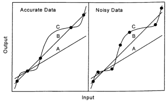
The principle of parsimony dictates that the simpler model should generally be chosen. Simpler models are more generalizable and less likely to overfit the data, ensuring that the signal is captured while minimizing the influence of noise. Importantly, the residuals (the difference between observed and model-predicted values) from a simpler model often still contain useful information, which can be analyzed further to refine predictions. This highlights that simpler models, while not perfectly fitting the data, often strike the optimal balance between accuracy and generalizability.
Advantages and Disadvantages of Simpler Models
- Vulnerability: Simpler models have fewer parameters and less flexibility, which makes them more vulnerable to falsification. According to Popper’s philosophy, this is a desirable quality because it ensures models are testable and scientifically robust.
- Comprehensive Description: While simpler models aim to provide a more comprehensive and interpretable description of the system, they can sometimes be overly descriptive, capturing patterns that may not be meaningful or applicable beyond the dataset.
- Complex Models: More complex models offer greater flexibility and can fit the data more closely, which can be advantageous for postdiction but detrimental for prediction. This flexibility can also introduce ambiguity, as multiple complex models might fit the data equally well.
The goodness of fit of a model to the data determines its quality for postdiction, but parsimony ensures improved prediction by avoiding overfitting. Model selection becomes particularly challenging with noisy data because the signal-to-noise ratio is lower, and simpler models may struggle to distinguish between the two.
Trade-offs in Model Selection
Model selection requires careful consideration of multiple factors, including:
- Number of model parameters versus size of the dataset: A model with too many parameters risks overparameterization, where it fits the noise rather than the signal. Conversely, a model with too few parameters may oversimplify and fail to capture important patterns in the data.
- Statistical Power: There is always a trade-off between the complexity of a model and the statistical power to detect true effects. A model that is too complex reduces power, while a simpler model improves robustness but may miss subtle signals.
To address these issues, it is often necessary to estimate the accuracy of the data using replication (repeated experiments) or simulation. Additional knowledge about the system being studied can also aid in selecting the most appropriate model. Ultimately, the principle of parsimony—choosing the simplest model that adequately describes the data—ensures a balance between overfitting and underfitting, leading to better generalization and more accurate predictions.
Statistical Terminology
In statistical analysis, several measures exist to evaluate signal and noise, as well as to quantify how well data align with a particular model. These measures provide insight into the accuracy, precision, and efficiency of statistical models. The Root Mean Square (RMS) is a measure of data variability and is defined as: \[\begin{equation} \sqrt{\frac{1}{n}\sum_{i=1}^{n}x_i^2} \end{equation}\]
It captures the magnitude of deviations in the data. The Sum of Squares (SS) measures the total variability of data around the mean and is expressed as: \[\begin{equation} \sum_{i=1}^{n}(X_i-\bar{X})^2 \end{equation}\]
The Mean Square further refines this measure by dividing the SS by the degrees of freedom (d.f.), which depend on the number of model parameters. For example, a model with three parameters such as \(y = abx + cx^2\) has 3 degrees of freedom.
The Signal-to-Noise Ratio quantifies the strength of the signal relative to noise: \[\begin{equation} \frac{SS_{signal}}{SS_{noise}} \end{equation}\]
A higher ratio indicates that the signal dominates over noise, allowing for clearer interpretations. Another critical measure is Statistical Efficiency, which compares the variance of two estimators (\(T_1\) and \(T_2\)) relative to the true value \(\theta\): \[\begin{equation} e(T_1,T_2) = \frac{E[(T_2-\theta)^2]}{E[(T_1-\theta)^2]} = \frac{\text{Variance of data around true values}}{\text{Variance of model around true value}} \end{equation}\]
A higher statistical efficiency reflects a model’s superior ability to extract meaningful information from noisy data. However, a significant challenge lies in the fact that noise is often unknown and difficult to quantify, which complicates precise model evaluation. Understanding and applying these statistical measures helps identify models that balance parsimony—maximizing signal extraction while minimizing unnecessary complexity and noise.
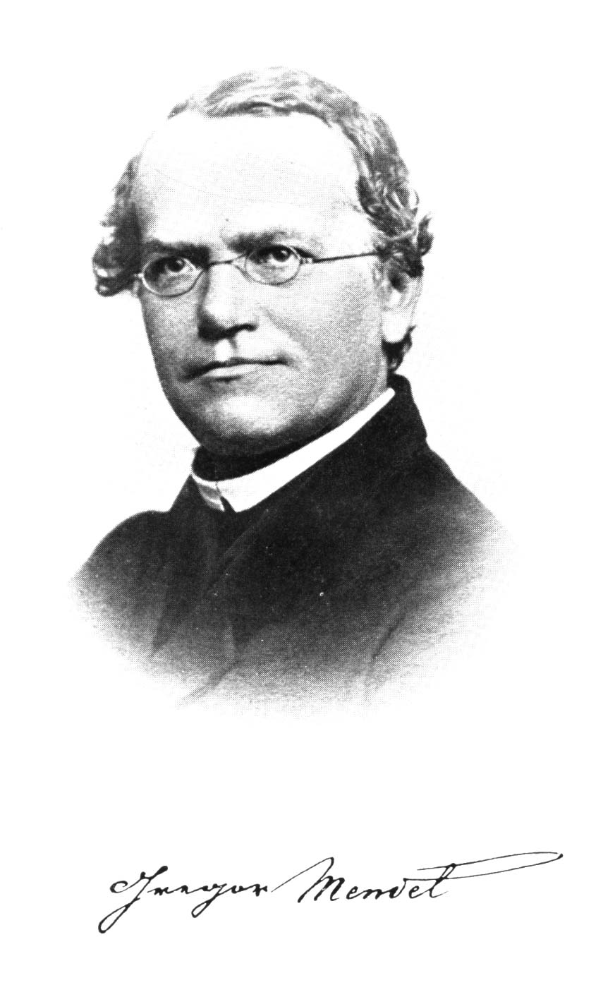
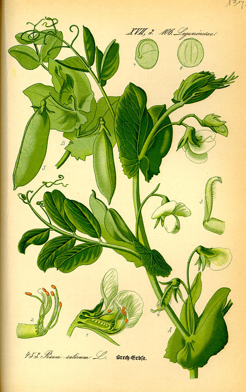
An example of parsimony from genetics
The application of the parsimony principle can be demonstrated with Mendel’s peas.

| Trait | Ratio |
|---|---|
| Round : wrinkled shape | 2.96 : 1 |
| Yellow : green endosperm | 3.01 : 1 |
| Dark : white seed coats | 3.15 : 1 |
| Inflated : constricted seed pods | 2.95 : 1 |
| Green : yellow unripe pods | 2.82 : 1 |
| Axial : terminal flower positions | 3.14 : 1 |
| Tall : short plants | 2.84 : 1 |
| Average | 2.98 : 1 |
| Dominance : Recessivity | 3 : 1 |
Mendel’s conclusion: “…an average ratio of 2.98:1 or 3:1”
Summary
- Strong inference, as proposed by Platt, is a scientific method that involves creating alternative hypotheses, designing crucial experiments to test these hypotheses, and sequentially refining scientific understanding through iterative testing.
- Models can take various forms (deterministic/stochastic, static/dynamic, quantitative/qualitative) and are crucial tools for scientists to represent and investigate complex biological and scientific processes.
- The principle of parsimony (Occam’s Razor) suggests that among theories that fit the data, scientists should choose the simplest one, balancing explanatory power with model complexity to avoid overfitting.
- Understanding the difference between signal and noise is critical in scientific research, with scientists aiming to develop models that capture true underlying trends while minimizing the impact of random variations or experimental errors.
- Model selection involves careful consideration of trade-offs between model complexity, statistical power, and predictive accuracy, with the ultimate goal of creating models that can generalize effectively and make meaningful predictions about scientific phenomena.
Key concepts
Further reading
There is large literature on the relationship of models and data. Here is a selection of some excellent resources.
- Gauch (2003), Chapter 8 - The lines of arguments in this chapter was mostly taken from this book
- Hugh G. Gauch (2012), Chapter 10 - A more accessible and readable account of chapter 8 of Gauch’s 2002 book.
- Gauch (2006) - Another summary of Gauch’s arguments used for this chapter
- Bodner et al. (2021) - A very good and simple introduction into mathematical modeling
Additional readings:
- Hilborn and Mangel (1997) The Ecological Detective - Confronting Models with Data. Princeton University Press. Chapter 2. - A classical and easily unterstandable introduction to the topic.
- Diggle et al. (2011) Statistics and the Scientific Method - An Introduction for Students and Researchers. Oxford University Press. Chapter 2. - Also a very good introduction
- Box (1976) Science and Statistics J. Am. Stat. Ass. 71:791-799. - Nice philosophical introduction (http://www-sop.inria.fr/members/Ian.Jermyn/philosophy/writings/Boxonmaths.pdf)
Study questions
- How does the concept of strong inference, as described by Platt, differ from traditional scientific methodologies, and what are the key steps in applying this approach to scientific research?
- Explain the relationship between theories, hypotheses, and models. Using the example of nitrogen fertilization and plant yield from the document, demonstrate how these scientific constructs can be used to develop and test scientific understanding.
- What is the principle of parsimony (Occam’s Razor), and how does it guide scientists in model selection? Discuss both its historical development and its practical applications in scientific research.
- Compare and contrast the concepts of prediction and postdiction in scientific modeling. How do these approaches differ, and what challenges do they present in developing accurate scientific models?
- Analyze the concept of signal and noise in scientific research. How do scientists distinguish between meaningful information and random variations, and what statistical techniques can be used to improve the signal-to-noise ratio?
- Discuss the trade-offs involved in model selection, considering factors such as model complexity, statistical power, and predictive accuracy. Using examples from the chapter, explain how scientists have to balance these competing considerations when developing scientific models.
In class exercises
Constructing a predictive model
Assume that your task is to construct a predictive model for the relationship between nitrogen fertilization and crop yield.
The task is based on the following premises:
- Theory: Nitrogen is required for plant growth because it is an essential component of proteins.
- Hypothesis: More nitrogen applied during plant growth leads to a higher yield.
- Null hypothesis: There is no effect of nitrogen fertilization on plant growth.
In the lecture notes, we already presented three possible models, which are shown in Figure 10.
Please discuss the following questions:
- One could imagine a fourth model, which describes the increase of yield with higher levels of nitrogen fertilization. Can you draw a curve for this model and describe its behaviour in words?
- Assume that you are doing a field trial to evaluate to which model your data fit the best. Can you describe in words (without a mathematical formula) which approach you would take to fit each of the three (or four) models above to your data as shown in Figure ref:fig:withdata? How could you use the approach to both estimate the model parameters and find the best fitting model?
Thinking about parsimony
Ontological and epistemiological aspects of parsimony
What are the ontological and epistemological aspects of parsimony? In which respect are both simplicity and complexity true characteristics of “nature”?
If you think about the above models:
- Can you identify an ontological parsimony and an epistemiological parsimony in the relationship between nitrogen fertilization and yield?
- If you differentiate between science and application (farming): When do you think it is advantageous to step away from parsimony and embrace complexity in both domains? When is it sufficient to choose a parsimonius approach?
Relationship between parsimony and experimental design
Do you think there is a relationship between the extent of parsimony and experimental design?
Think about the role of experimental and other (i.e. environmental) errors in a field trial. What are the requirements to make a parsimonious model more robust with respect to noise that inevitably is present in field trials (and other types of experiments)?