Show the code
```{r}
1 + 1
```This computer lab introduces a key concept of reproducible research, namely computational notebooks. We use the Quarto publishing system, which allows to write notebooks in the simple Markdown format, combine code from multiple programming languages and allows a simple export into multiple output formats (e.g., HTML, PDF, DOCX, etc) for different uses (presentations, reports, scientific publications).
Note: The following tutorial is adapted from a tutorial by Prof. Karl Broman.
git.1 See, for example https://sembr.org/
In this module we explore the recently published quarto system.
Quarto enables you to weave together content and executable code into a finished document that can be exported to multiple formats. To learn more about Quarto see https://quarto.org. A very concise introduction to Quarto can be found in the 2nd edition of the open access book R for Data Science.2
When you click the Render button a document will be generated that includes both content and the output of embedded code. Y ou can embed code like this:
```{r}
1 + 1
```You can add options to executable code like this
The echo: false option disables the printing of code (only output is displayed) in the export of the notebook to another format. For a list of available options, see:
On the Quarto website, find out which code chunk option hides the code in the report.
quarto render to convert these documents into PDF and other formats.quartoIn scientific data analysis the result is usually a written report (e.g., a thesis or a scientific publication) which describes the rationale, methods and the results. All persons involved in such a project document their work for further use.
Quarto and plain RMarkdown allow to write some reports that can present the analysis and results in different formats.
Such data analysis reports are ideally reproducible documents. If an error is discovered, or if some additional subjects are added to the data, you can just re-compile the report and get the new or corrected results (versus having to reconstruct figures, paste them into a Word document, and further hand-edit various detailed results).
The key tool for doing this is Quarto, which allows you to create a document that is a mixture of text and some chunks of code.
When the document is processed by ´Quarto`, chunks of R (or Python or Julia) code will be executed, and graphs or other results inserted. This approach to data analysis and programming is know as literate programming.
An alternative solution (solely for R) is to use knitr. knitr allows you to mix basically any sort of text with any sort of code, but it is recommended to use R Markdown, which mixes Markdown with R. Markdown is a light-weight mark-up language for text.
In the following, however, we show the process for Quarto.
Within R Studio, click File → New File → Quarto Document and you’ll get a dialog box like this:
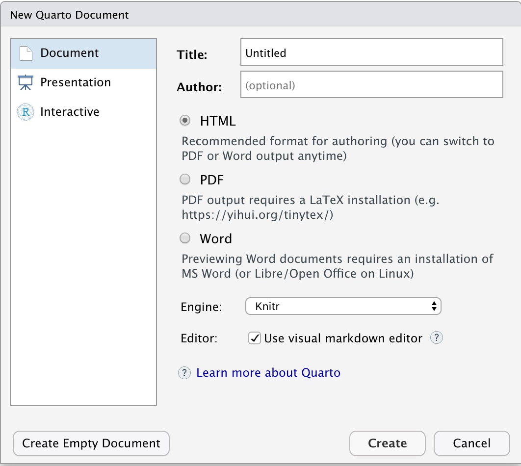
You can use the default (HTML output), but you should give your document a title.
The initial chunk of text contains instructions for R: you give the thing a title, author, and date, and tell it that you’re going to want to produce html output (in other words, a web page).
You can delete any of those fields if you don’t want them included. The double-quotes aren’t strictly necessary in this case. They’re mostly needed if you want to include a colon in the title.
RStudio creates the document with some example text to get you started. Note below that there are chunks like
{r}
summary(cars)
``
These are chunks of R code that will be executed by knitr and replaced by their results as described below.
Also note the web address that’s put between angle brackets (< >) as well as the double-asterisks in **Knit**. This is Markdown.
Markdown is a system for writing web pages by marking up the text much as you would in an email rather than writing html code. The marked-up text gets converted to html, replacing the marks with the proper html code.
For now, let’s delete all of the stuff that’s there and write a bit of markdown.
You make things bold using two asterisks, like this: **bold**, and you make things italics by using underscores, like this: _italics_.
You can make a bulleted list by writing a list with hyphens or asterisks, like this:
* **bold** with double-asterisks
* _italics_ with underscores
* `code-type` font with backticks
or like this:
- **bold** with double-asterisks
- _italics_ with underscores
- `code-type` font with backticks
Each will appear as:
(I prefer hyphens over asterisks, myself.)
You can make a numbered list by just using numbers. You can use the same number over and over if you want:
1. bold with double-asterisks
1. italics with underscores
1. code-type font with backticks
This will appear as:
You can make section headers of different sizes by initiating a line with some number of # symbols:
# Title
## Main section
### Sub-section
#### Sub-sub section
You compile the R Markdown document to an html webpage by clicking the “Render” button in the upper-left.
You can make a hyperlink like this: [text to show](http://the-web-page.com).
You can include an image file like this: 
You can do subscripts (e.g., F2) with F~2 and superscripts (e.g., F2) with F^2^.
If you know how to write equations in LaTeX, you’ll be glad to know that you can use $ $ and $$ $$ to insert math equations, like $E = mc^2$. For example,
$$y = \mu + \sum_{i=1}^p \beta_i x_i + \epsilon$$will be shown as:
\[y = \mu + \sum_{i=1}^p \beta_i x_i + \epsilon\]
Markdown is interesting and useful, but the real power comes from mixing markdown with chunks of R (or Python, or Julia) code. This is R Markdown. When processed, the R code will be executed; if they produce figures, the figures will be inserted in the final document.
The main code chunks look like this:
{r load_data}
gapminder <- read.csv("~/Desktop/gapminder.csv")
``
That is, you place a chunk of R code between {r chunk_name} and ``. It’s a good idea to give each chunk a name, as they will help you to fix errors and, if any graphs are produced, the file names are based on the name of the code chunk that produced them.
.qmd fileWhen you press the “Render” button, the Quarto document is processed and converted to HTML, PDF or Word file. the R code is executed (depending on the settings) and replaced by both the input and the output; if figures are produced, links to those figures are included.
The Markdown and figure documents are then processed by the tool pandoc, which converts the Markdown file into an html file, with the figures embedded.
There are a variety of options to affect how the code chunks are treated.
#| echo: false to avoid having the code itself shown.#| results: hide to avoid having any results printed.#| eval: false to have the code shown but not evaluated.#| warning: false and #| message: false to hide any warnings or messages produced.#|fig.height and #|fig.width to control the size of the figures produced (in inches).Note: The following is outdated. Update to Quarto!
So you might write:
{r load_libraries, echo=FALSE, message=FALSE} library("tidyverse") library("knitr") ``
Often there will be particular options that you’ll want to use repeatedly; for this, you can set global chunk options, like so:
{r global_options, echo=FALSE}
knitr::opts_chunk$set(fig.path="Figs/", message=FALSE, warning=FALSE,
echo=FALSE, results="hide", fig.width=11)
``
The fig.path option defines where the figures will be saved. The / here is really important; without it, the figures would be saved in the standard place but just with names that begin with Figs.
If you have multiple R Markdown files in a common directory, you might want to use fig.path to define separate prefixes for the figure file names, like fig.path="Figs/cleaning-" and fig.path="Figs/analysis-".
You can make every number in your report reproducible. Use r and for an in-line code chunk, like so: `r` `round(some_value, 2)` . The code will be executed and replaced with the value of the result.
Don’t let these in-line chunks get split across lines.
Perhaps precede the paragraph with a larger code chunk that does calculations and defines things, with include=FALSE for that larger chunk (which is the same as echo=FALSE and results="hide").
I’m very particular about rounding in such situations. I may want 2.0, but round(2.03, 1) will give just 2.
You can also convert R Markdown to a PDF or a Word document. Click the little triangle next to the “Knit HTML” button to get a drop-down menu. Or you could put pdf_document or word_document in the header of the file.
Tip: Creating PDF documents
Creating .pdf documents may require installation of some extra software. If required this is detailed in an error message.
In the previous computer lab (R introduction) you had to solve some exercises. Now, convert the solution of the exercises into an html report using R Markdown. Try to:
Add a title, author, and date
Create a section for each exercise
Name each chunk of code
If a plot is produced:
fig.height and fig.widthPlay with chunk options to see the effects (echo=FALSE, results="hide", ..)
At the end of the report, create a section with a numbered list with the exercises you found more difficult.
OPTIONAL: Show a result of HWfreq function from exercise 11.0.1 (e.g. using a p frequency of 0.2) as a markdown table (as shown in the solutions handout). Hint: https://rmarkdown.rstudio.com/lesson-7.html
At least convert exercises: 5.1.1, 10.3.1 and 11.0.1